Data Access Framework Exercise - Hazard Services

Retrieving and Viewing Data using Data Access Framework (DAF)

Purpose:

This jobsheet will go through a few of the fundamental steps in creating a data request using DAF and viewing the data.

Tasks:

Open a terminal window. You can do this by right clicking on the desktop and clicking "Open Terminal". NOTE: You must be on a Linux workstation with AWIPS.
Open Python by typing "python" and pressing enter. You will see ">>>" at the beginning of the line when Python is ready to receive commands.

Start by importing the necessary libraries. Copy and paste each line below into your terminal window, pressing enter between each one to load the library.

from dynamicserialize.dstypes.com.raytheon.uf.common.dataquery.requests import RequestConstraint
from ufpy.dataaccess import DataAccessLayer
from datetime import datetime, timedelta
import matplotlib.pyplot as plt
import numpy as np

Let's take a look at what data types are available in AWIPS (i.e. grid, obs, radar, maps, hydro, etc.). Copy and paste the following lines into your terminal (still in Python), again, one at a time.
```
availtypes = DataAccessLayer.getSupportedDatatypes()
print availtypes
```
1. You should see the available data types in the form of a list. Verify that 'hydro' is an option, as this will be the data type we will use. The hydro data is the river gage data from the AWIPS hydro database.
Now let's create a data request. We will add items to the request in subsequent steps. Copy and paste each of the following two lines (separately) into your terminal window and press enter to run each one:
```
request = DataAccessLayer.newDataRequest()
request.setDatatype('hydro')
```
1. The first line initiates the new request. The second line tells the request that it will be accessing the "hydro" data type from the list of available types that was printed before.
Next, run the following line to add a constraint to the request. This specifies that "height" is a filter for "table":
```
request.addIdentifier('table', 'height')
```
1. "addIdentifier" is basically a way to refine search results in the request.
The following two lines are used to query possible location IDs and parameters, allowing you to see what is available from your data type.
```
availloc = DataAccessLayer.getAvailableLocationNames(request)
availparam = DataAccessLayer.getAvailableParameters(request)
```
1. Optional step: enter the command "print availloc" (without the quotes) to see a print out of all possible gages/location IDs. Alternatively, you can print a slice of the list, such as "print availloc[0:20]" to see just the first 20 location IDs in the list and not clutter your terminal window.
Type the line "print availparam" and press enter to see a list of parameters that are available in the 'hydro' data type. You should see an output similar to this:
```
['lid', 'pe', 'dur', 'ts', 'extremum', 'obstime', 'value', 'shef_qual_code', 'quality_code', 'revision', 'product_id', 'producttime', 'postingtime']
```
Now lets make the final assembly of DAF request, using a single location id and the 'value' and 'obstime' columns, which are a couple of the parameters listed in the previous output. Copy and paste the following lines into your python terminal window one at a time and replace ALKP1 with one of the gages of your choice from your availloc list.
```
request.setLocationNames('ALKP1')
request.setParameters('value', 'obstime')
```
1. NOTE: You can also use "availloc" here instead of a single location ID, however it may take significantly longer. The same applies for the second line: You can use "availparam" instead of listing specific parameters, however expect a longer processing time.
Now let's pass our final request object to the getGeometryData method by entering the following line:
```
response = DataAccessLayer.getGeometryData(request)
response.sort(key = lambda x: x.getNumber('obstime'))
```
1. The variable "response" has all of the data that we requested. If you print response, you will see a bunch of "<ufpy.dataaccess... >" objects, which is not helpful unless you have an IDE that can query their contents. Now we will want to access that data to view or process.
Enter the following line:
```
print response[0].getNumber('value')
```
1. This will print the first item in response, but just the NUMBER associated with the response object, which looks something like the 2.83ft stage height from ALKP1 shown below. If you want to see the type of the value in this object, try using "getType" instead of "getNumber". If the type returns "string", you can use "getString" to extract the string from the object.
2. Note: You can replace the "0" in the response[0] array with "1" for the next stage height in the array and "-1" for the last stage height in the array.
```
2.83 
```
Now let's compare the stage height in the previous step to a Timeseries plot of the hydro database.
1. Open the Hydro perspective in CAVE and be sure that station locations are visible (Point Data Control is loaded from the MapData menu).
2. If you know the location of the station that you used in the previous step (e.g. ALKP1), then right click and hold on this gage to see a list of menu options and choose "Timeseries" to see a time series plot appear.
  1. NOTE: if you cannot find the correct gage location on the map, choose any gage location, right click and hold on the gage and choose Timeseries, and in the "Time Series Control" panel that appears, use the scroll bar to find and select your gage ID (e.g. ALKP1) and select the Graph button on the bottom of the Time Series Control to plot the time series.
3. If you click and drag anywhere on the graph, you can see a readout of the value at your cursor (shown at the top of the graph). Place your cursor over the first dot in the time series and you will see that it has a value of 2.83 ft, just like the value we printed in the terminal (the first gage height value in our values list).
  1. Note: In the Time Series Control Panel, you may need to set your "Beginning Time" back quite a bit earlier to see the first data point available in the time series.
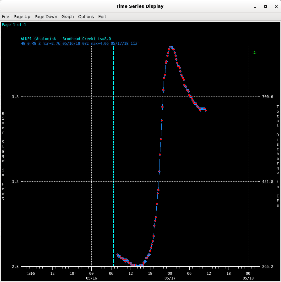
4. 1. NOTE: You can ZOOM in on the graph by going to "Graph" in the menu bar at the top of the window and clicking "Zoom" --> "Set", where you can then select an area to zoom in to.
In the next few steps, we are going to create a script that will allow us to run a series of commands without having to copy and paste each one. This will help us get the data into a more basic form used to view and graph by setting up a loop through the existing "<ufpy.dataaccess...>" objects. To begin, open a NEW terminal window (not Python).
Type nano DAFScript.py and press enter. (If you are familiar with another command line text editor, such as vim, feel free to use that instead of nano.) This will open a text editor in the terminal window you are working in.

Copy and paste the following set of commands, being sure to keep correct indentation, matching what is shown here. Be sure to change the river gage LID to the one chosen in previous steps (see "request.setLocationNames" line in script).

from dynamicserialize.dstypes.com.raytheon.uf.common.dataquery.requests import RequestConstraint
from ufpy.dataaccess import DataAccessLayer
from datetime import datetime, timedelta
import matplotlib.pyplot as plt
import numpy as np

request = DataAccessLayer.newDataRequest()
request.setDatatype('hydro')
request.addIdentifier('table', 'height')
request.setLocationNames('ALKP1') #CHANGE THIS to the appropriate river gage for your CWA
request.setParameters('value', 'obstime')


#Example of how to add a constraint to the request - making sure value is greater than 0
valueconstraint = RequestConstraint.new('>', 0) 
request.addIdentifier('value', valueconstraint)


response = DataAccessLayer.getGeometryData(request)
response.sort(key = lambda x: x.getNumber('obstime'))

gage_heights = []
gage_obs_times = []
for i in range(len(response)):	
    gage_heights.append(response[i].getNumber('value'))
    ts = response[i].getNumber('obstime')
    ts /= 1000 #obstime in terms of milliseconds, convert to seconds
    ts_string = datetime.utcfromtimestamp(ts).strftime('%Y-%m-%d %H:%M:%S')
    gage_obs_times.append(ts_string)

plt.plot(range(len(gage_obs_times)), np.array(gage_heights))
plt.ylabel("Gage Height (ft)")
plt.xticks(range(len(gage_obs_times))[::150], gage_obs_times[::150], rotation=90)
plt.axhline(y=3.8, color='r')
plt.show()

When you are ready to save the file, press ctrl+O, which will write the contents to the file. You will see "File Name to Write: DAFScript.py" - press enter to verify that this is correct. Then, press ctrl+X to exit the file and return to your standard terminal window.
For notes on the purpose of each remaining line of this script (those which have not already been reviewed above), take a look at the following steps. To skip ahead to running this script, see step 18.
1. Sometimes missing values are filled with large negative numbers such as -9999. To avoid these data points, we set up a constraint before calling the final response which allows us to only grab values that are greater than 0 (i.e. avoid missing values).
```
#Example of how to add a constraint to the request - making sure value is greater than 0
valueconstraint = RequestConstraint.new('>', 0) 
request.addIdentifier('value', valueconstraint)	
```
2. Calling the response is a necessary step. Note, however, that the response will not be returned in the correct time-sorted order. Because of this, we have to sort the responses based on the parameter we choose, which in this case is 'obstime'.
```
response = DataAccessLayer.getGeometryData(request)
response.sort(key = lambda x: x.getNumber('obstime'))
```
3. The following two lines set up empty lists for the gage height values and the times associated with them:
```
gage_heights = []
gage_obs_times = []
```
4. Now we will set up the loop with the following line:
```
for i in range(len(response)):
```
  1. This says for the index "i" in the range of the length of the response array (i.e. 0 to the length of response), do the following. This begins a loop.
5. Within the loop and the if statement are the following lines:
```
        gage_heights.append(response[i].getNumber('value'))
        ts = response[i].getNumber('obstime')
        ts /= 1000 #obstime in terms of milliseconds, so this line helps
        ts_string = datetime.utcfromtimestamp(ts).strftime('%Y-%m-%d %H:%M:%S')
        gage_obs_times.append(ts_string)
```
  1. The final line ("gage_obs_times.append...") simply takes the new string form of obstime and appends it to the empty list we set up before the loop.
  2. Lines 2-4 (lines starting with "ts") are steps to get the "obstime" value into a human readable format for viewing purposes by first extracting the obstime value from the tuple, changing it from milliseconds to seconds, and then using a datetime method (from the datetime library we imported) to put the date in a string of the form "Year-month-day hour:minute:second".
  3. The first line ("gage_heights.append...") is appending the current gage height value (as we noted in step 11) to the empty list "gage_heights". On each loop, the new value will be added to the end of the list.
6. We are then ready to plot this data! We use the following line to set up the initial pyplot object:
```
plt.plot(range(len(gage_obs_times)), np.array(gage_heights)
```
7. The following lines make the data more meaningful:
```
plt.ylabel("Gage Height (ft)")
plt.xticks(range(len(gage_obs_times))[::150], gage_obs_times[::150], rotation=90)
plt.axhline(y=3.8, color='r')
plt.show()
```
  1. These lines set up x- and y-axis labels, the x-labels are the times we gathered in the loop. We have set them to label only every 150th tick mark, because otherwise the x-axis would be too crowded to read (try changing "150" to a different number, or removing the "[: : 150]" altogether to see what happens). You will likely need to adjust this number to get a good fit.
  2. The next line ("plt.axhline...") plots a red horizontal line at y=3.8. This number can be changed to whatever is appropriate, and may help identify certain thresholds with the river gage heights.
  3. plt.show() is the final line that puts all of the plt commands together and forms a figure.
To run this script: From your terminal window, type python DAFScript.py and press enter. This says to use python to run the script. You should see a figure pop up (depending on the amount of data plotted, it may take a minute).
1. NOTE: You will need to CLOSE the open figure window if you want to re-run this script from the terminal.
That's it! Feel free to play around with the options by editing your script and re-running it. You can also add the commands we used to set up the DAF data request to the script and change variables such as the station location, data type, and more.

BONUS: If you want to try learning about other data types and the getGeometryData method, try running this code, which explores the "warning" data type. (Keep the pre-existing imports, as before).

request = DataAccessLayer.newDataRequest()
request.setDatatype('warning')
request.setLocationNames('KLWX') #CHANGE THIS: change LWX to appropriate CWA for you - keep "K" in front
request.setParameters('ugczones')

response = DataAccessLayer.getGeometryData(request)
print "length of response: ", len(response)


#Try changing the number after response to anything within the length printed above to see other polygons
poly = response[0].getGeometry()

#Uncomment the line below to see the geometry lat/lon values printed out
#print poly


x,y, = poly.exterior.xy
plt.plot(x,y)
plt.show()

Previous: Completely Removing Hazard Types	Focal Point Basics Table of Contents	Next: Data Access Framework Exercise (Part 2)

Data Access Framework Exercise - Hazard Services

Focal Point Basics Jobsheets

Retrieving and Viewing Data using Data Access Framework (DAF)

Purpose:

Tasks: