Data Access Framework Exercise (Part 2) - Hazard Services

Focal Point Basics Jobsheets

DAF Jobsheet Part 2 (Radar and Grid Data)

Purpose:

This jobsheet is a continuation of the last DAF jobsheet, now focusing on retrieval of grid data.

Tasks:

Let's take a look at some radar data in AWIPS to get a feel for the data we will be retrieving. Open a new, BLANK CAVE editor and load One Hour Precip from one of your dedicated radars. FOR FOCAL POINT WORKSHOP: Look for the KLWX radar under dial radars (found in the Radar menu), and choose One Hour Precip from the KLWX Precip menu.
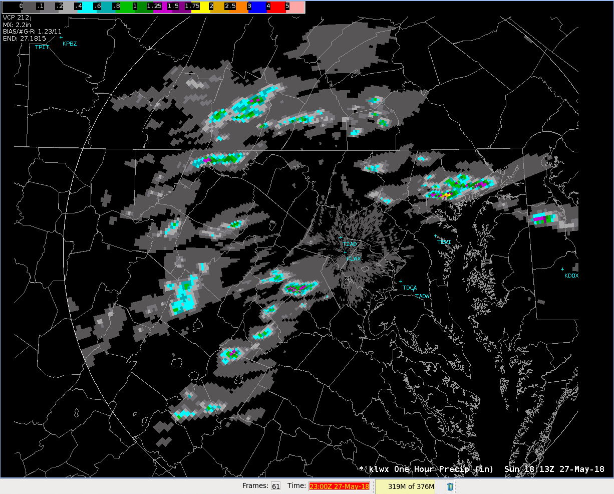
Click through the frames and find a time with some data. Leave AWIPS open in the background while completing the following steps.
Open a terminal window. You can do this by right clicking on the desktop and clicking "Open Terminal".
Type nano Grid_DAFScript.py and press enter. (If you are familiar with another command line text editor, such as vim, feel free to use that instead of nano.) This will open a text editor in the terminal window you are working in and create a new file with this name in your current location.

Copy and paste the following set of commands, being sure to keep correct indentation, matching what is shown here:

from dynamicserialize.dstypes.com.raytheon.uf.common.dataquery.requests import RequestConstraint
from ufpy.dataaccess import DataAccessLayer
from datetime import datetime, timedelta
import matplotlib.pyplot as plt
import numpy as np
import sys

#######
# This script is used to play with/test grid data in AWIPS


availtypes = DataAccessLayer.getSupportedDatatypes() #no argument needed here
#print availtypes #if you want to see what data types are available, uncomment this line

###################### USER INPUTS ###########################
datatype = 'radar'

loc = "klwx"

parameter = "One Hour Precip"

selected_time = "2018-05-27 18:13" #enter time in string form that matches time in CAVE

##############################################################

request = DataAccessLayer.newDataRequest()
request.setDatatype(datatype) #telling it which plugin to access
request.setLocationNames(loc) # TIP: can also use *availloc to request ALL locations, BUT might take a very long time
request.setParameters(parameter) # TIP: can also use *availparam here to request ALL parameters, BUT might take a very long time


# Next two lines are used to query possible location IDs and parameters and times
availloc = DataAccessLayer.getAvailableLocationNames(request) # After running, print availloc to show possible gauge/loc IDs
availparam = DataAccessLayer.getAvailableParameters(request) # After running, print availparam to show possible columns
availtimes = DataAccessLayer.getAvailableTimes(request)


print "\nNum. of available times: ", len(availtimes)



ind = []
print "Selected time: ", selected_time
print "Time matches: "
for i in range(len(availtimes)):
	if str(availtimes[i])[0:16] == selected_time:
		print availtimes[i]
		ind.append(i)
                break

else: #if no matching times are found, exit the script
        sys.exit("\nNo data at the selected time. Please select another time.\n")


time = availtimes[ind[0]:ind[0]+1] #must be list

num = 0

# pass our final request object to the getGridData method...
response = DataAccessLayer.getGridData(request, time) #time must be a list, not a single value


	

print "\nParameter: ", response[num].getParameter()
unit = response[num].getUnit()
print "Unit: ", unit
data = response[num].getRawData()
data[np.where(data<0)] = np.nan


if unit == "m":
	data = data*39.37 #convert from meters to inches to compare to CAVE display (x-hr precip shown in inches in AWIPS)
	unit = "in."
elif unit == "m^3*s^-1*km^-2":
        data = data*91.8 #(convert from cubic meters/set/sq. km to cfs/smi as shown in AWIPS)
        unit = "cfs/smi"
elif unit == "m^3*s^-1":
        data = data*35.315
        unit = "cfs"



if datatype == 'radar':
        azimuths = np.radians(np.linspace(0,360,360))
        zeniths = np.arange(0,np.shape(data)[0],1) #number of range gates, evenly spaced 
        r, theta = np.meshgrid(zeniths, azimuths) 
        values = np.random.random((azimuths.size, zeniths.size))


        #Plot on polar plot
        fig = plt.figure()
        ax = fig.add_subplot(111, polar=True)
        plt.contourf(theta, r, data[::-1,:].T)
        ax.set_theta_direction(-1)
        ax.set_theta_offset(np.pi/2)
        ax.set_rgrids([20,40,60,80,100], labels = ["40 km", "80 km", "120 km", "160 km", "200 km"])
        ax.set_rlabel_position(120)
        plt.title("{} for {} at {}".format(parameter, loc, time[0]))

else:
        lat_lon = response[num].getLatLonCoords()
        lons, lats = response[num].getLatLonCoords()    
        fig = plt.figure()
        ax = fig.add_subplot(111)
        plt.contourf(lons, lats, data)
        plt.title("{} at {}".format(parameter, time[0]))



clb = plt.colorbar()
clb.ax.set_ylabel(unit)

plt.show()

You will need to change a few variables to apply this script to the data you have.
1. Change radar_loc to the radar chosen in AWIPS with available data. (FOR FOCAL POINT WORKSHOP: use klwx radar as shown in code, since localization-specific radars are not available. The LWX database is available for this exercise)
2. Change selected_time to the product time frame (not CAVE clock) that you have open in AWIPS (this will be used to compare your plotted output to the data shown in AWIPS).
When you are ready to save the file, press ctrl+O, which will write the contents to the file. You will see "File Name to Write: Grid_DAFScript.py" - press enter to verify that this is correct. Then, press ctrl+X to exit the file and return to your standard terminal window.
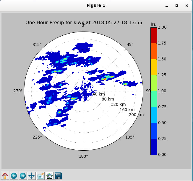
To run this script, type "python Grid_DAFScript.py" and press enter. This tells the terminal to use Python as the program to open and run the file. You should see a figure pop up (depending on the amount of data plotted, it may take a minute).
1. NOTE: You will need to CLOSE the open figure window if you want to re-run this script from the terminal.
The data plotted on the figure should match the data at the selected time in AWIPS. Use sampling to see the azimuth and range to determine that the values and locations of heaviest rainfall match up between the two. (Note: values not available in sampling - use the colorbar for estimates on your figure.)
- Sampling is "on" by default in the pop-up plot, just look to the bottom right corner of the figure for the readout.
- Zoom in on the features by clicking the cross button (4th button from the left) and then right click and drag anywhere on the figure.
- There is a section at the bottom of this jobsheet reviewing details of how this code works.
That's it! Now you are familiar with the commands to access radar precip estimates using the DAF. With this, you can include things like radar precip estimates in your modifications to recommenders and megawidgets. After the Bonus step below there is a breakdown of this code to help you understand how each part works.

BONUS: Now that you are familiar with the script, try making some changes to the user input variables to plot something else. For example, let's plot MRMS CREST Unit Streamflow:

In CAVE:
1. Go to CONUS view
2. Open the MRMS Menu --> FLASH products --> Crest Unit Streamflow
3. Find a time with a good amount of data
In Grid_DAFScript.py:
1. Change datatype to 'grid'
2. Change location to 'MRMS_1000'
3. Change parameter to 'QPECrestUStreamflow' (Later, also try 'QPECrestStreamflow' for fun!)
4. Update the selected_time variable in the script with the product time in CAVE.
5. Save the script and run it again.
You should see a pop-up figure displaying the MRMS CREST Unit Streamflow data matching that in the CAVE window.

There are a lot of potential uses for important parameters such as CREST Unit Streamflow in hydrological megawidget and recommender enhancements. This jobsheet has introduced you to how to access the data. As you investigate the structure of the python recommender files and megawidgets, you can look for ways to incorporate this type of data in future enhancements. The CREST data used here is grid, and there are many other types of grid parameters (e.g. model QPF) which can be beneficial for hydro recommender and megawidget enhancements. The process to follow will be:

Load the data in CAVE → If you can see data in CAVE, you should be able to retrieve it using the script.
Identify the parameter name → To get this, follow the inline code review described below with a few additional lines added to the code.
Identify a time from CAVE and update the script before running it

Please take a look at the following additional steps which break down each block of this code. These steps may help if you intend to try new things which are not part of the guided exercise.

The first section of code (shown below) is used to create a new request and refine the request based on a specific data type, location, and parameter (chosen by user). If you would like to see available datatypes, uncomment the line below which starts with "#".

availtypes = DataAccessLayer.getSupportedDatatypes() #no argument needed here
#print availtypes #if you want to see what data types are available, uncomment this line

###################### USER INPUTS ###########################
datatype = 'radar'

loc = "klwx"

parameter = "One Hour Precip"

selected_time = "2018-05-27 18:13" #enter time in string form that matches time in CAVE

##############################################################

request = DataAccessLayer.newDataRequest()
request.setDatatype(datatype) #telling it which plugin to access
request.setLocationNames(radar_loc) # TIP: can also use *availloc to request ALL locations, BUT might take a very long time
request.setParameters(parameter) # TIP: can also use *availparam here to request ALL parameters, BUT might take a very long time

[OPTIONAL] If you would like to see all available locations for a datatype, try putting these lines right before the "USER INPUTS" line:

request = DataAccessLayer.newDataRequest()
request.setDatatype('radar') #tell it which datatype to look at
availloc = DataAccessLayer.getAvailableLocationNames(request)
print availloc
availparam = DataAccessLayer.getAvailableParameters(request)
print availparam

This will allow you to see ALL possible locations and parameters before narrowing down the request with specific options. Use this if you'd like to experiment with other parameters and are not sure what to use. (NOTE: Be aware that not all data may be available, even if it says a parameter is available.)

The next section (shown below) provides information about the request. Since we defined the request before calling "getAvailableLocationNames" and "getAvailableParameters", these will return only the items we requested as options. If you want to see everything available to add to the request, put these lines above the request creation. Available times, however, is important to keep after the request creation, since otherwise you will get a list of times that don't all have associated data for the parameter.
```
availloc = DataAccessLayer.getAvailableLocationNames(request) # After running, print availloc to show possible gauge/loc IDs
availparam = DataAccessLayer.getAvailableParameters(request) # After running, print availparam to show possible columns
availtimes = DataAccessLayer.getAvailableTimes(request)

print "\nNum. of available times: ", len(availtimes)
```
The next section (shown below) uses the user-selected time to search for matching times in the dataset, then puts it into a form that is appropriate for the request (i.e. a list rather than a single object). If the loop completes without finding a matching time, the code will end and give the user a message that no times match the selected time, allowing them to re-run the script rather than getting a python error in the following step.
```
ind = []
print "Selected time: ", selected_time
print "Time matches: "
for i in range(len(availtimes)):
    if str(availtimes[i])[0:-3] == selected_time:
        print availtimes[i]
        ind.append(i)

else: #is no matching times are found, exit the script
    sys.exit("\nNo data at the selected time. Please select another time.\n")

time = availtimes[ind[0]:ind[0]+1] #must be list	
```
The next section (shown below) passes the request and the selected time to the "getGridData" method. This is the step that ultimately retrieves the data. num = 0 is just set in case our response is larger than 1, i.e., if more than 1 time was entered for "time".
```
num = 0

# pass our final request object to the getGridData method...
response = DataAccessLayer.getGridData(request, time) #time must be a list, not a single value
```
The next few lines (shown below) provide the user with some useful information about the response (i.e. the data retrieved), such as which parameter was requested (e.g. One Hour Precip), and what the unit is of that parameter. There is also a line removing placeholder values that are negative so that only "good" data is plotted. The "if/else" statement is in place to convert the data to appropriate units, since the raw data for most parameters is in Metric units, however AWIPS displays the data in US Standard. A few other units are included in the if/else statement for conversion, but be aware that not all unit conversions are included, so if you plot data with any other units, it may not match what the CAVE display shows.
```
print "\nParameter: ", response[num].getParameter()
unit = response[num].getUnit()
print "Unit: ", unit
data = response[num].getRawData()
data[np.where(data<0)] = np.nan

if unit == "m":
    data = data*39.37 #convert from meters to inches to compare to CAVE display (x-hr precip shown in inches in AWIPS)
    unit = "in."
elif unit == "m^3*s^-1*km^-2":
    data = data*91.8 #(convert from cubic meters/set/sq. km to cfs/smi as shown in AWIPS)
    unit = "cfs/smi"
elif unit == "m^3*s^-1":
    data = data*35.315
    unit = "cfs"
```

Since radar data is based on azimuth and range rather than lat/lon coordinates found in most grid data types, a special section is set up to prepare a plot if the data type is radar. This section includes a few steps of pre-processing to get a plot correctly set up before plotting the radar data from the response. For all other grid data (the "else" block), we retrieve the lat/lon coordinates associated with the data to set up the plot. Most of these lines are used to format the plot (e.g. make sure the polar plot reflects meteorological N/S/E/W, set location and labels for the radials, etc.). These settings can and may need to be changed if other parameters are plotted, or based on user preference.

if datatype == 'radar':
    azimuths = np.radians(np.linspace(0,360,360))
    zeniths = np.arange(0,np.shape(data)[0],1) #number of range gates, evenly spaced 
    r, theta = np.meshgrid(zeniths, azimuths) 
    values = np.random.random((azimuths.size, zeniths.size))


    #Plot on polar plot
    fig = plt.figure()
    ax = fig.add_subplot(111, polar=True)
    plt.contourf(theta, r, data[::-1,:].T)
    ax.set_theta_direction(-1)
    ax.set_theta_offset(np.pi/2)
    ax.set_rgrids([20,40,60,80,100], labels = ["40 km", "80 km", "120 km", "160 km", "200 km"])
    ax.set_rlabel_position(120)
    plt.title("{} for {} at {}".format(parameter, loc, time[0]))


else:
    lat_lon = response[num].getLatLonCoords()
    lons, lats = response[num].getLatLonCoords()    
    fig = plt.figure()
    ax = fig.add_subplot(111)
    plt.contourf(lons, lats, data)
    plt.title("{} at {}".format(parameter, time[0]))

Finally, we plot the data that is retrieved, and add a colorbar along with colorbar label.
```
clb = plt.colorbar()
clb.ax.set_ylabel(unit)
plt.show()
```

Previous: Data Access Framework Exercise	Focal Point Basics Table of Contents