Tutorial: Using NDFD gridded data in a GIS Environment (Shapefiles and Floating Point Grids)

 

Why bring NDFD grids into a GIS?

One of the most attractive components of the National Digital Forecast Database is the geospatial nature of the data. The database is based on a 5km national grid that covers the Continental U.S. and separate grids that cover Hawaii, Alaska, the U.S. Virgin Islands, and Puerto Rico. Each 5km grid cell has forecast information so that a point specific forecast can be generated for any cell based on geographic coordinate location. Besides being able to just view the grids using algorithms to create graphics of the gridded information, more advanced users may want to perform analysis with gridded data to answer some real-world problems. Bringing the NDFD gridded files into a GIS enables the user to not only display the forecast elements with other georectified datasets such as satellite imagery, aerial photographs, and planimetric layers such as political boundaries, road networks, buildings, etc…, but also to query the data and use it for geospatial analysis. The result is essentially a real-time and forecast decision support tool for making critical decisions based on various weather elements. This is the case for marine interests as well, as the NDFD grid extend offshore several miles and deliver wave and wind information. Using the NDFD data in a GIS gives the flexibility to deal with either Raster versions of the NDFD grids (floating point grids), or vector versions (ESRI shapefiles) as well as other formats that are just recently becoming importable into GIS like NetCDF files and GRADS. The best way to illustrate the power of using NDFD grids in a GIS can best be presented via a use case scenario given below.

Using NDFD grids for pre-Hurricane landfall decision making

During the 2004 hurricane season NDFD forecast elements were used to display experimental forecast elements such as wind speed, wave heights, and quantitative precipitation forecasts along with hurricane forecast tracks in a map format that was used by DHS/FEMA for risk analysis at the FEMA Region IV Regional Operation Center and Disaster Field Office. For hurricanes Charley, Frances, Ivan, and Jeanne maps were created showing NDFD forecast elements overlaid on relevant political boundaries, roads, shoreline, and major population centers. The elements gave DHD/FEMA risk analysts an idea of the spatial coverage and intensity of forecast winds and wave heights. These maps were used to create the Presidential Briefing Package in which DHS/FEMA briefs the executive branch on potential damages that will be incurred from the approaching storm so as to pre-secure federal resources for response and aid through a presidential disaster declaration. This is an example of how having the NDFD grids converted to GIS significantly benefited the decision making process for weather driven natural disasters such as hurricanes. See Figure 1 and 2 below.

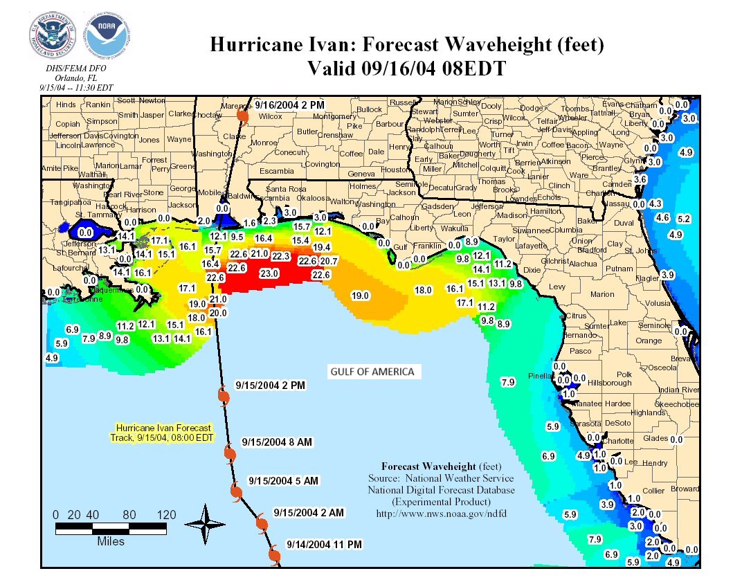
Figure 1: Forecast wave height along the shore of the Gulf of Mexico during Hurricane Ivan.

Figure 2: Forecast wind speed along the shore of the Gulf of Mexico during Hurricane Ivan.

Download the data

1. Instructions for downloading the data

1. In the graphical user interface (GUI) tkdegrib, click on the Download tab.
2. Expand the NDFD data set folder.
3. Choose the sector (or region) of interest and expand the file. Data for each weather element can be downloaded by highlighting the sector file, or individual weather elements can be downloaded by holding down the Control key on the keyboard and highlighting one or more elements.
4. After all the selected data are highlighted, click on either the Download by ftp button or the Download by http button (either will work) at the bottom of the window (Figure 3). Once the downloading begins, there will be an indication in the Message Window that it is working. Also, after the download button is clicked, the progress bar (the light blue bar near the bottom of the window) will start at 0 percent and show progression as the data download. Note: The progress bar will say 100 percent before any downloading has taken place.

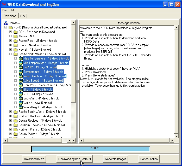
Figure 3: In this example, the user needs data from specific weather elements within the Pacific Northwest sector. Only the needed weather elements are highlighted, rather than the entire sector, and the user is about to click on the Download by http button.

2. Convert the data to an ESRI shapefile

1. When the data are finished downloading, click on the GIS tab.
2. Browse through the sectors for the downloaded data in the top left corner of the window.
3. Double-click on a specific weather element in the top right corner, and it should fill out the inventory chart below.
4. Select the data set in the inventory chart to be converted to a shapefile (Figure 4).

Note: For more information on the inventory chart, see the Degrib: Man Pages and Full Tutorial. A similar document is also available in a portable document format. NDFD Tkdegrib and GRIB2 Data Download Tutorial (PDF).

 

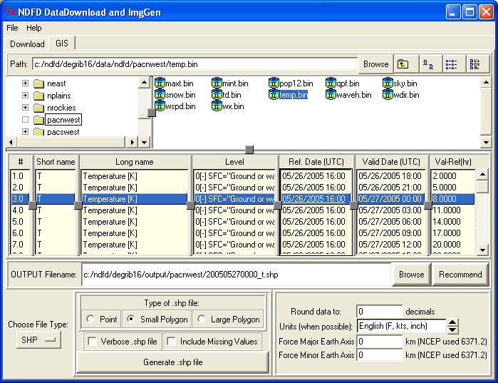
Figure 4: In this example pacwest (Pacific Northwest) sector is expanded. The temp (temperature) file has been expanded and a data set is highlighted in the inventory chart. The shapefile this user wants to create is the temperature of the Pacific Northwest on 5/27/2005 at 12:00 a.m., which is 8 hours from the time the weather was forecasted.

 

e. Click on the Choose File Type menu at the bottom left corner of the window and choose SHP (Figure 5).

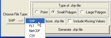Figure 5: Choose SHP from the Choose File Type drop-down menu.

 

f. Manually type the output file name into the OUTPUT Filename dialog box or click the Recommend button to have tkdegrib choose one (Figure 6).

Figure 6: When tkdegrib recommends a file it stores it on the local drive in the ndfd/degrib16/output folder. Inside that folder is a folder for each of the sectors. The generated shapefile will be in the corresponding sector folder. In the example above the temperature data (_t) is from the Pacific Northwest sector (pacnwest). The data are for 05/27/2005 at 12:00 a.m.

 

g. Now choose the Type of .shp file (Point, Small Polygon, or Large Polygon).

Note: For more information on types of shapefiles download the NDFD Tkdegrib and GRIB2 Data Download Tutorial (PDF).

h. Check the box for Verbose .shp file if the values for latitude, longitude, and X and Y are needed. A non-verbose shapefile will generate point identification and data, but not the latitude, longitude, and X and Y (Figure 7).

A.	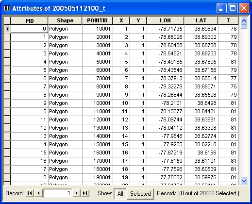B.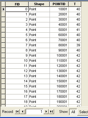
Figure 7: A verbose .shp file imports the point identification (POINTID) and data (T, or temperature), as well as the X and Y and latitude (LAT) and longitude (LON) (A). A non-verbose .shp file only imports the point identification and data (B).

 

i. The default values for the box in the bottom right corner for Round data to will default to a number when Recommend for Output File is clicked. Most weather elements will have a default of 0. The default for Units (when possible) can be accepted or changed, depending on personal preferences. The values for both Force Major Earth Axis and Force Minor Earth Axis are more advanced options and should be left as 0 for general purposes (Figure 8).

Note: The Round data to value will show its default when the Recommend button is complete. Most of the weather elements will default as 0; the exceptions are snow and waveh, which will default as 1, and qpf, which will default as 2.

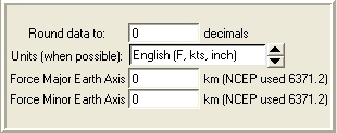Figure 8: Depending on preference, the default values can be accepted for Round data to and Units. The Earth Axis options are for more advanced options.

 

j. Then click the Generate .shp file button at the bottom center of the window.

3. Import an ESRI shapefile into ArcGIS:

1. Open a new window in ArcMap.
2. Click on the Add Data button  and navigate to the previously selected location of generated .shp file.
3. Highlight the file and click the ADD button (Figure 9).

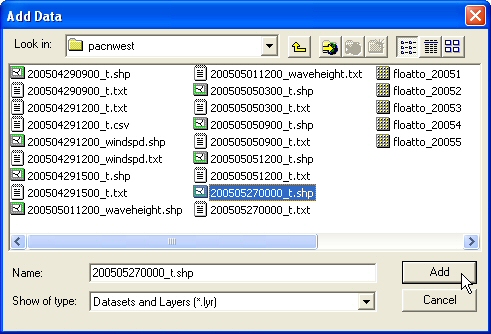Figure 9: In this example, a shapefile for temperature in the Pacific Northwest sector was generated and placed in the pacnwest folder. Navigate to the shapefile and highlight the shapefile. Click the Add button.

 

d.The shapefile will now appear in the Display view on the left side of the window, and the Map view  will appear in the right side of the window. Both the Display tab or Table of Contents and the Map view tab should already be selected (Figure 10).

 

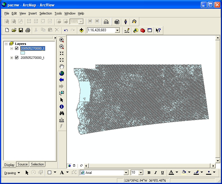
Figure 10: In this example, a large polygon shapefile was added into ArcMap. The data represent the temperature (_t) of the Pacific Northwest (pacnwest) sector for 05/27/2005 at 12:00 a.m. When a shapefile is imported into ArcMap, the symbology is defaulted as one symbol and one color.

4. Load Legends into ArcMap to view GRIB2-derived shapefiles:

1. Double-click on the shapefile in the Display view (or right-click and scroll down to Properties) of ArcMap.
2. In the Layer Properties dialog, click on the Symbology tab.
3. Click on the Import button in the top left corner (Figure 11).

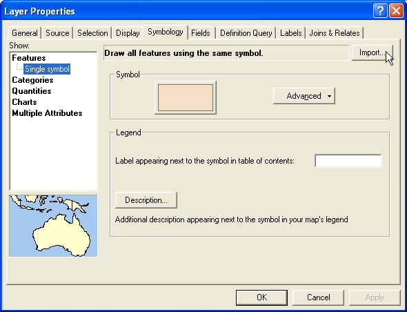
Figure 11: In the example above, the Symbology tab is selected and the user is going to import a standard legend into ArcMap.

d. In the Import Symbology dialog box, select Import symbology definition from an ArcView 3 legend file (*.avl) and click the browse button (Figure 12).

Figure 12: After selecting Import symbology definition from an ArcView 3 legend file, browse to the folder where they are located.

 

e. Navigate to the /ndfd/degrib16/arcview/ folder.

f. Select the /point_legend or /poly_legend, depending on which type of shapefile was generated, and highlight the individual weather element that the shapefile addresses.

g. Click the Open button (Figure 13).

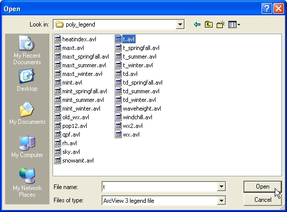Figure 13: In the previous examples, the weather element data that were downloaded were for temperature, and the type of shapefile generated was a large polygon. In this example, the corresponding .avl file is needed. In the poly_legend folder (since a polygon shapefile was generated) select the temperature (t) .avl.

 

h. In the Import Symbology dialog box, under What do you want to import? select Complete symbology definition and click OK (Figure 14).

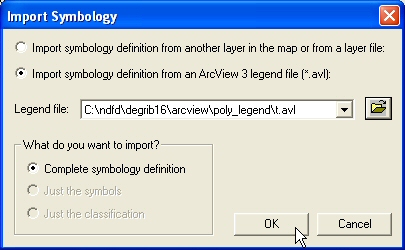Figure 14: Notice in this example that the Legend file is a poly_legend\t.avl, since that is the type of .shp file generated in previous steps. After selecting the legend file, select Complete symbology definition and click OK.

 

i. Accept the Value Field default value in the Import Symbology Matching Dialog box and click OK (Figure 15).

 

Figure 15: In this example, the value field is T, since the shapefile generated is for temperature and the legend file is for temperature. This value will be a default, according to which .avl file is imported into ArcMap.

 

j. In the Layer Properties dialog, there should be different colors for the Symbol and different numbers for the Value. Click OK (Figure 16)

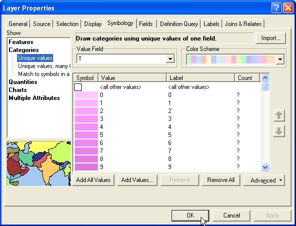
Figure 16: The ArcView standard symbology is now imported into ArcMap and applied to the shapefile.

 

k. Notice the symbology is now applied to the shapefile in both the Display view and the Map view (Figure 17).

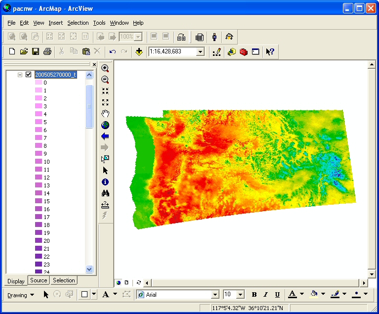
Figure 17: Notice the difference between the symbology in this example and the example in Figure 8. The ArcView standard symbology has been imported into ArcMap and applied to this example.

5. Convert a message to ESRI Spatial Analyst or GrADS file format:

1. In the GUI tkdegrib, click on the GIS tab.
2. Browse for the downloaded file in the upper left corner of the window.
3. Double-click on a specific weather element in the top right corner of the window, and it should fill out the inventory chart in the mid-section of the window.
4. Click the desired message in the inventory chart (Figure 18).

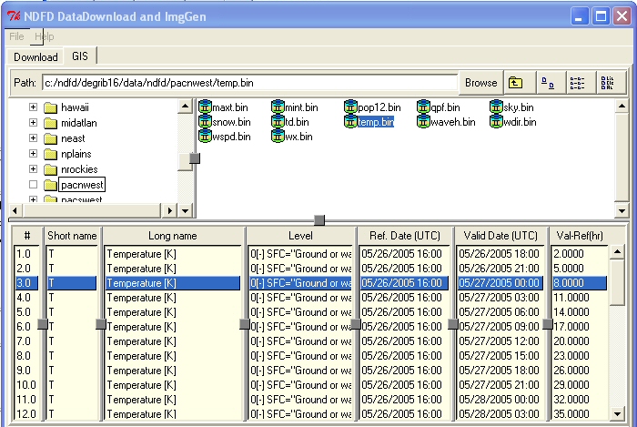
Figure 18: In the example above, Pacific Northwest is expanded. The temperature weather element has been double-clicked to expand its data set. The user wants to generate a file of the temperature of the Pacific Northwest on 5/27/2005 at 12:00 a.m, which is 8 hours from the time the weather was forecasted.

 

e. Click on Choose File Type in the lower left section of the window and choose FLT from the drop-down menu (Figure 19).

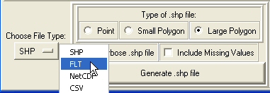Figure 19: Choose FLT from the Choose File Type drop-down menu to generate a float file.

 

f. In the Grid drop-down menu, choose one of the three options: Projected: Original GRIB; Coverage: Nearest Point; or Coverage: Bi-Linear.

Note: For more information see full tutorial (LINK).

g. To create the GrADS .ctl file, check the box for Create GrADS .ctl file (Figure 20).

Figure 20: Choose a type of grid to fit preferences from the Grid drop-down menu. Select Create GrADS .ctl file.

 

h. The other three options (Start at Upper Left, use NDFD Weather code, and M.S.B. First) are more advanced options and do not need to be selected for general purposes.

i. In the OUTPUT Filename dialog box, type the output file name or click Recommend to have tkdegrib choose one (Figure 21).

Figure 21: When tkdegrib recommends a file, it stores it on the local drive in the ndfd/degrib16/output folder. Inside that folder is a folder for each of the sectors. The generated .flt will be in the corresponding sector folder. In the example above, the temperature data (_t) is from the Pacific Northwest sector (pacnwest). The data are for 05/27/2005 at 12:00 a.m.

 

j. The default values for the box in the bottom right corner for Round data to and Units (when possible) can be accepted or changed, depending on personal preferences. The values for both Force Major Earth Axis and Force Minor Earth Axis are more advanced options and should be left as 0 for general purposes (Figure 22).

Note: The Round data to value will show its default when the Recommend button is complete. Most of the weather elements will default as 0; the exceptions are snow and waveh, which will default as 1, and qpf, which will default as 2.

Figure 22: Depending on preference, the default values can be accepted for Round data to and Units. The Earth Axis options are for more advanced options.

 

k. Click the Generate .flt file button at the bottom of the window.

6. Open an FLT file in ArcGIS:

a. Open a new window in ArcMap and click on the ArcToolbox icon . This will open the ArcToolbox window (Figure 23).

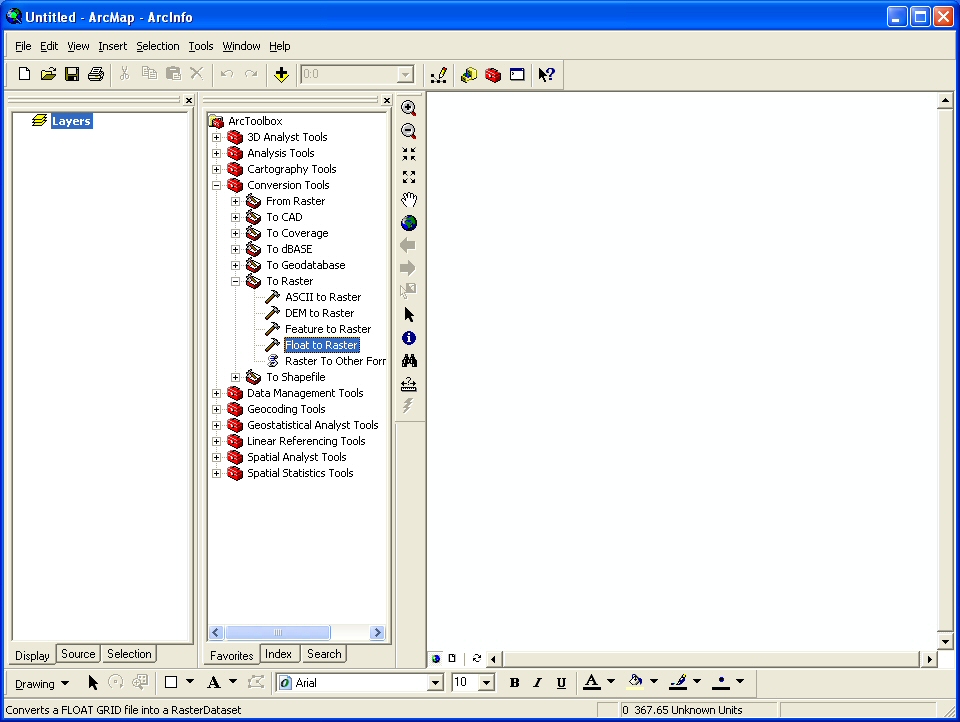
Figure 23: Click on the ArcToolbox icon to open ArcToolbox. In Arc 9, ArcToolbox will open within the ArcMap window.

 

b. Expand the Conversion Tools option in the Favorites window.

c. Expand the To Raster option. Then double-click on the Float to Raster selection (Figure 24).

Figure 24: In the ArcToolbox menu, expand Conversion Tools, and then expand To Raster. Double-click Float to Raster.

d. In the Float to Raster window, click on the browse button next to Input floating point raster file (Figure 25).

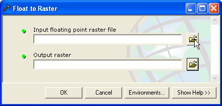Figure 25: Click on the browse button to locate the .flt file to be converted to raster.

 

e. Find the .flt file which was generated from the NDFD DataDownload tool and open it so that it appears under Input floating point raster file (Figure 26).

Figure 26: Locate the .flt file to be converted to raster. It will be found where the OUTPUT file was saved in step 5i. Highlight it and click Open.

 

f. The program should create an Output Raster location. Click OK (Figure 27).

Figure 27: The program will suggest an output location, which will probably be in the same location as the original .flt file. Click OK.

 

g. There will be an indication that the conversion is taking place and when it is finished. Click Close when it says "Completed" in the upper left corner (Figure 28).

Figure 28: This window will give an indication that the program has successfully converted the float file to a raster. Click Close when it says "Completed" in the upper left corner.

 

h. The new Float to Raster file is now a binary raster file that has been converted to a floating point grid and can be used for raster analysis in ArcGIS (Figure 29).

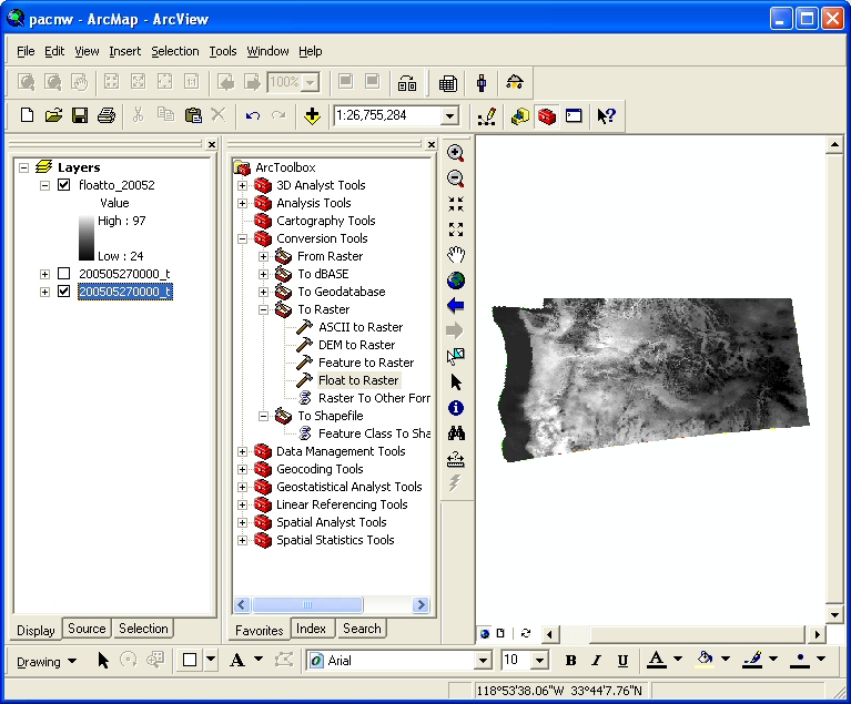
Figure 29: The .flt file of the Pacific Northwest was converted to a raster file so that it could used for raster analysis in ArcGIS.

Note: To print this page, choose the landscape orientation in the printer dialog box.

Return to top