The Volume menu has numerous ways of loading and displaying model grid data. Grid data is a unique data type in AWIPS because it supports displaying data as both graphics (e.g. contours) and images (color-filled layers). While the model data under the Volume menu is more for forecast applications than warning applications and are outside the scope of this RAC-oriented training, we will review some of the model grid data basics that support warning decision making.

The Volume menu contains many different groups of model parameter displays called Families that are tailored to each model. Under the Families section there are single panel family layouts and 4 panel family layouts with linked panel displays. Model families are typically a blend of graphic products (i.e. contours) and image products (i.e. color-filled displays) stacked on top of each other with product legends for each parameter. Many of the parameters are toggled off by default which makes the product legends darker. You you can toggle individual products on using a left mouse click on the product legend or by using the 1-9 numbers (and Shift + 1-9) on the keypad. Any model grid product loaded can be converted to a contour graphic or a color-filled image by right clicking on the product legend and selecting the appropriate submenu.

Most of the families in the Volume menu are standard forecast parameters like 500mb height and vorticity and mean sea-level pressure, but the families at the bottom of the menu support particular forecast problems (e.g. Convect, Surface, Winter)

The Volume Browser, Popup SkewT, and Standard Env Packages will be covered in separate sections.

The Volume Browser is a simple and robust model data loading tool that can be used to generate plan view plots, cross sections, time heights, variable versus height, soundings, and time series. The main types of products that can be loaded are found under the fourth menu on the upper left. In the last menu on the top you can load multiple frames of data products in time (e.g. 500mb heights each forecast hour) or space (geopotential height for each available vertical grid layer at a particular time).

Once you select a type of display along the top row of menus (e.g. Plan-view), you need to select a source, field, and plane for your product. The Sources menu contains traditional single-model volume sources like the NAM, pre-defined ensembles of data like the Global Ensemble Forecast System (GFS ensemble), and surface grids like the High-Resolution Precipitation Estimator (HPE).

The fields menu is where you can select a basic parameters like temperature and wind or more sophisticated severe weather parameters (under T-Storms) like CAPE. Radar data is one non-grid data type that is read in and converted from polar-format radar data to cartesian-format grid format where you can make graphics contours or image color-filled layers out of the data. Radar data is unique because there is no way to specify a particular radar from the VB menus, rather you set the cursor home to the location of the radar (via Tools button in VB or Tools button in D-2D) before you load the data. Having radar data in the Volume menu allow you to map radar fields to many different coordinate systems to combine with other model data.

The planes are where you can specify height coordinates such as pressure, theta (isentropic), height, temperature, or even radar tilts. One of the more commonly used planes is the surface which is located in the Misc Planes menu.

Once you have specified the proper source, field, and plane, if the data exists, an entry will show up in the bottom white box with check boxes next to the times in the forecast hours. If no data exists for the parameters you have specified, nothing will populate in the bottom white box. It can take some time and trial and error to identify the appropriate fields and planes for a given source, so a good strategy early on is to rely on local experts to learn from. 

Sometimes after entering in some of the parameter sections, you may notice that the VB will show you green boxes next to the menu items that are possible to load. It is good not to depend on menu statuses though, since this is a fairly complicated configuration tool, and the green boxes do not always show up, or do not always mean you have specified the correct source, field, and plane.

Once you have product identified in the bottom white box, select the product and click the Load button. Many models products will load as graphics, though you can convert a graphic to an image with a right click on the product legend.

Standard Environmental Data Package

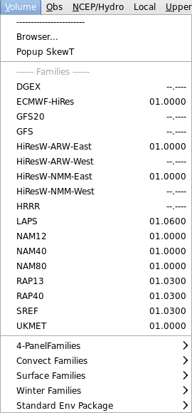
The Standard Environmental Data Package is one of the integrated radar environmental sampling tools in AWIPS. Loading the Standard Environmental Data Package from one of the standard model or observational input sources results in an overlay for elevation-based radar products where fields such as temperature and wind from the environment are mapped to the tilts of the radar data. The environmental sampling data are loaded from the Volume menu in the “Std Env Data Package” section. The data from this overlay can be accessed using the standard CAVE sampling feature. By default, the environmental data visible via sampling is:

• Wind speed and direction,
• Relative humidity, and
• Temperature.

Other environmental data are also part of the Standard Environmental Data Package, but they are toggled off by default:

• Pressure,
• Wet bulb temperature, and
• Equivalent potential temperature.

While these parameters are initially invisible overlays, they can be made visible. By default, the Density for all of these overlays is set to 0. By setting the Density to a non-zero value, the overlay contours become visible on the radar tilts.

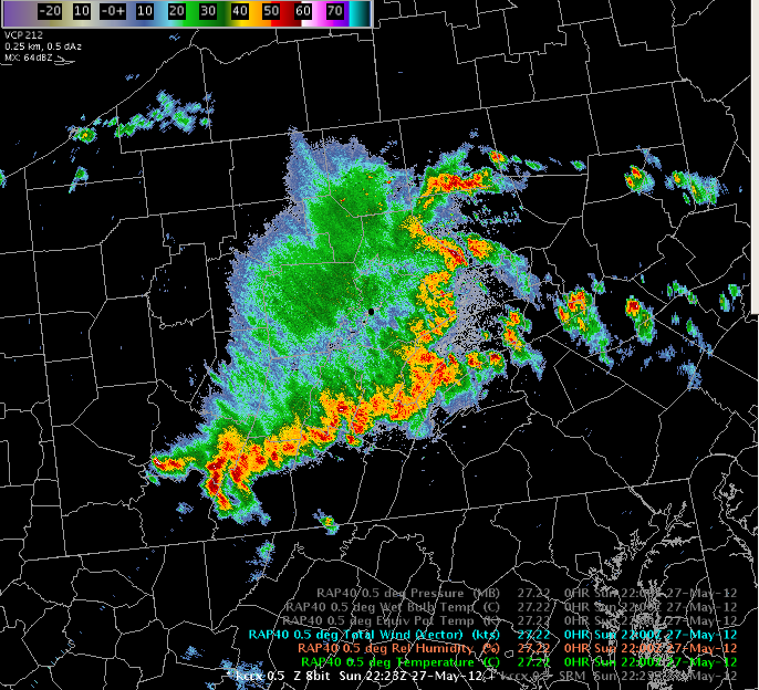
When using the Standard Environmental Data Package to integrate environmental data with your base radar data analysis, it’s important to remember that the data values shown are only valid for the center of the radar beam (e.g. while the center of the beam may be 0C the top may be -5C and the bottom may be 5C). In areas of poor radar sampling at long ranges with large beam volumes, radar and environmental interpretation is inherently more complex.

More information on the Standard Environmental Data Package can be found in  WES Exercise 3 Integrated Radar Environmental Sampling.

Pop-Up Skew-T

The other integrated radar environmental sampling tool available in AWIPS is the pop-up Skew-T window. The Skew-T window displays vertical profiles of environmental data at any point you are sampling. The profiles are dynamic and change as you move the cursor around the main display panel. The vertical profiles show the vertical temperature and dewpoint temperature profiles, the height of the current cursor location (indicated by a yellow dot if this is combined with base radar data), and the moist adiabatic curve for the LFC at that location.

To load the pop-up Skew-T window, you need to select the “Popup SkewT” menu item from the Volume menu. After performing this task, you will also need to select a data source for this application. To select a source, press and hold the Right Mouse Button in the background of the main display panel to access a context sensitive menu. In this menu, you’ll need to select the “Sample Cloud Heights/Radar SkewT” submenu and then select a data source from the submenu. It is also necessary to select right-click and hold on the background of the main display and select “Sample” if it is not already active. After performing this step, then the pop-up skew-T window will be visible.

When using the pop-up skew-T, it’s possible that the application window gets hidden behind the CAVE window. To avoid this problem, use the application window’s configuration menu (located in the upper left-hand corner of the window) and select the “On Top” menu item. Choosing this setting will make sure the pop-up Skew-T window is always the top level window, even if you are using the CAVE window. This way, you can easily analyze the data in both the CAVE window and in the Skew-T.

The Popup Skew-T provides a snapshot of the vertical environmental profiles while simultaneously analyzing radar data. While this application can be quite useful, there is a significant caveat that needs to be taken into consideration when using the pop-up Skew-T. While the popup Skew-T shows the height of the beam center in the window, it doesn’t provide any indication of the actual beam size at that location. Forecasters should realize, for storms located far away from the radar, that the volume the radar is sampling may be several thousand feet across. In these situations, the meaning of a single value like temperature or dewpoint at a point in the window is more ambiguous yet an inherent character of radar data.

The Popup SkewT also works over model forecast data, and it can allow you to dynamically roam the horizontal model forecasts with the vertical temperature and dewpoint profile.

More information on the pop-up Skew-T can be found in WES Exercise 3 Integrated Radar Environmental Sampling.