General Information about CAVE and the D2D Perspective
While the Advanced Weather Interactive Processing System (AWIPS) is composed of a large suite of programs, this training is going to focus mostly on the warning-related components of the Common AWIPS Visualization Environment (CAVE) and the Display in 2 Dimensions (D2D) perspective.
Redhat 7 Classic Gnome Desktop
On operational LX workstations, CAVE is run from a Redhat 7 Classic Gnome desktop. The Redhat 7 Classic Gnome desktop has been customized to behave uniquely for AWIPS, and this will be different than non-AWIPS machines.
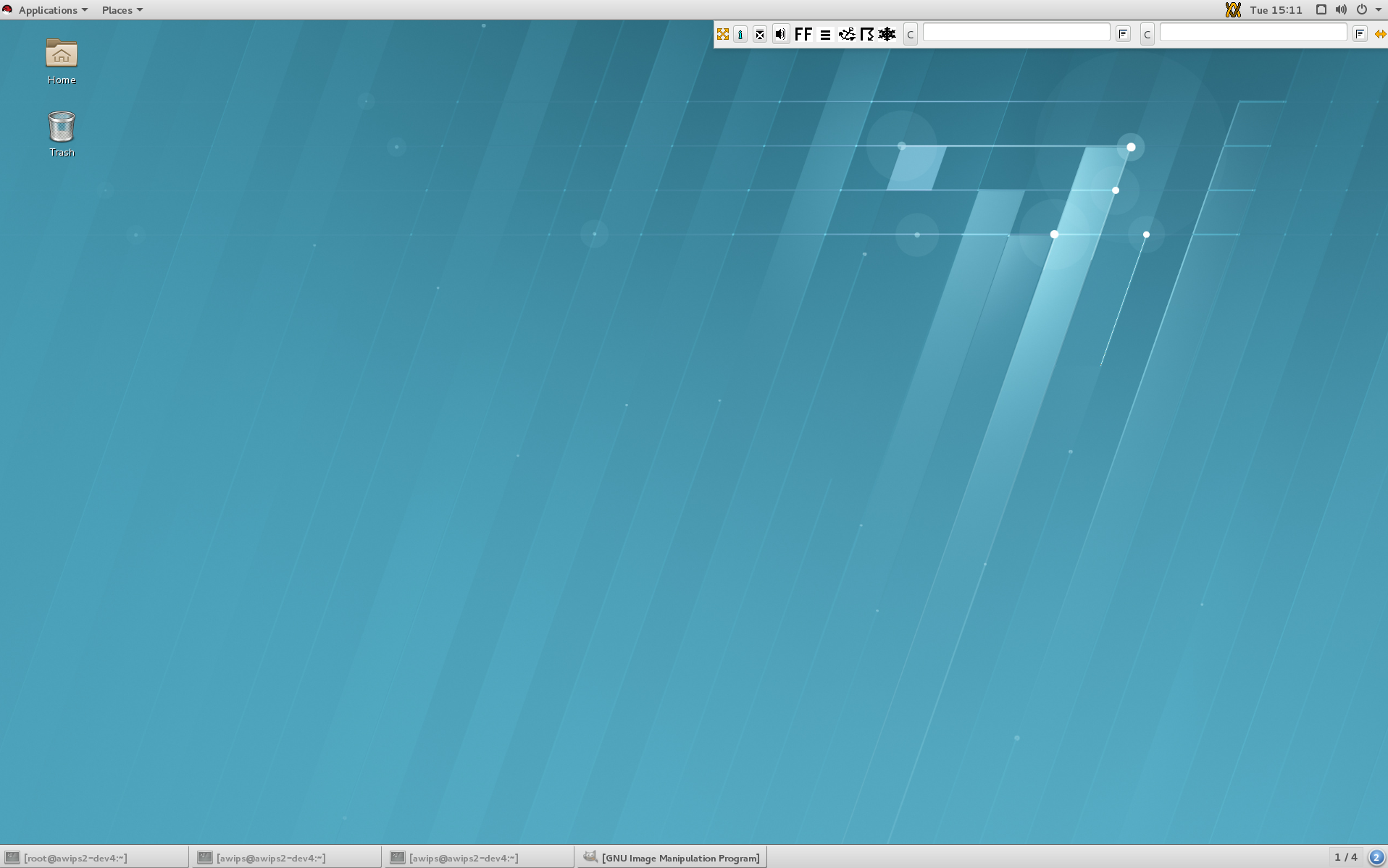
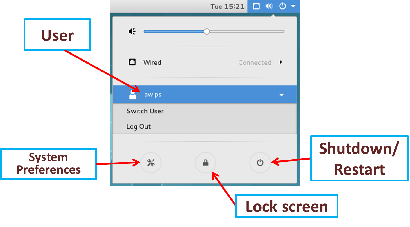
The logout window from the power button in the upper-right of one of monitors on the desktop is used to lock your screen, log out, and restart the workstation.
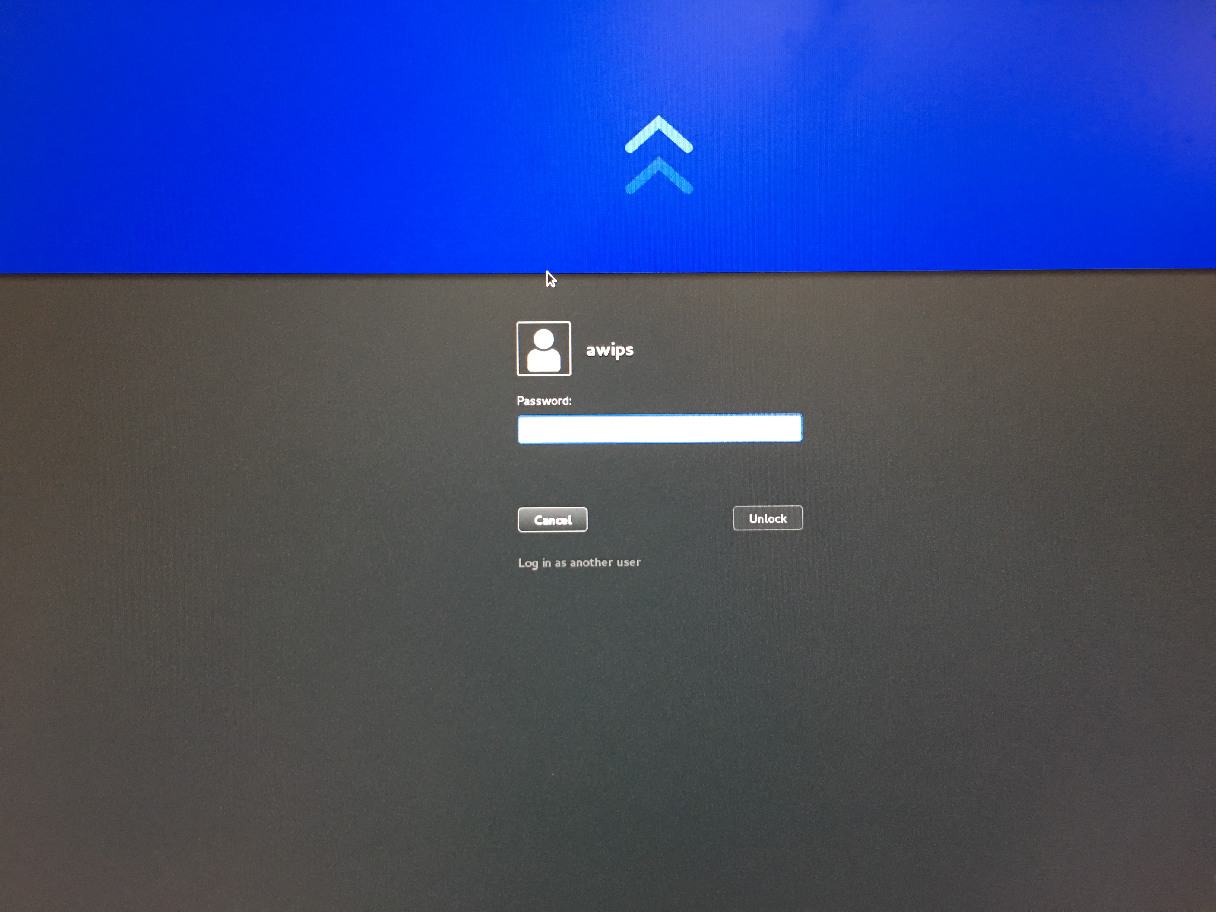
Note the screensaver doesn't respond to mouse clicks, but you can either use the keyboard to wake the screen saver or left mouse click and drag screen up (like swiping upward on a tablet).
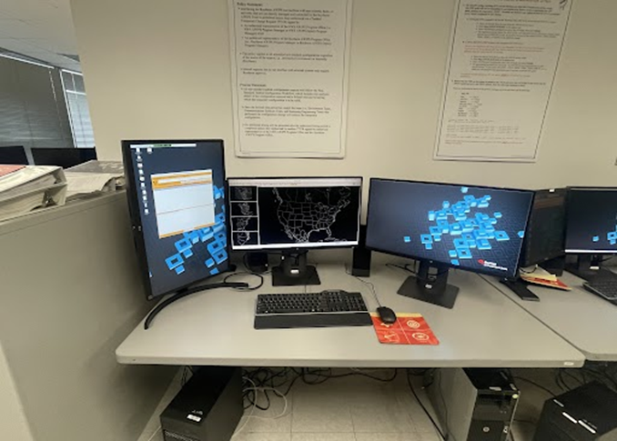
There are 3 monitors on an LX workstation on a shared desktop. These monitors can be configured with a portrait or layout orientation.
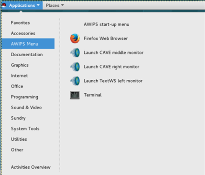
Cave is launched from the Applications-> AWIPS Menu on the upper-left part of one of the monitors on the desktop.
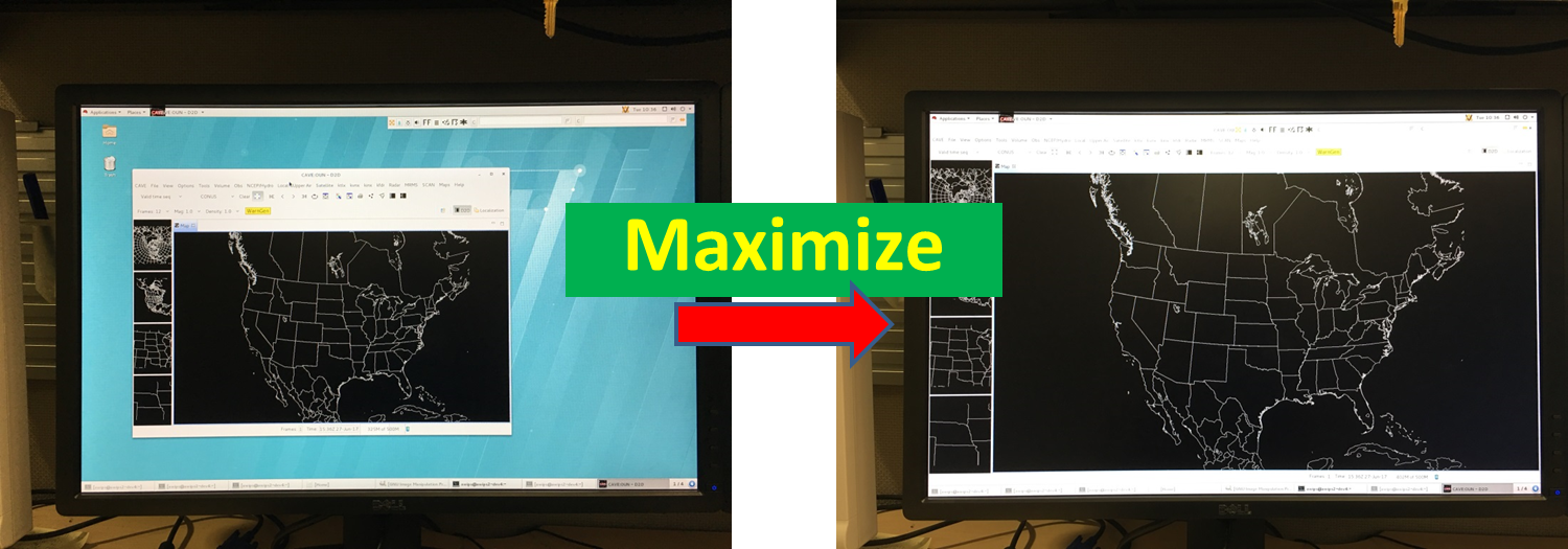
Maximizing display space is essential in AWIPS for many different windows, including CAVE. One tip is to use the maximize button in the upper-right part of the window to expand the window to fill the monitor.
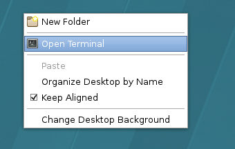
The middle monitor in AWIPS is unique in allowing a right click to generate a menu to launch applications like "Open Terminal".
CAVE and Perspective Display

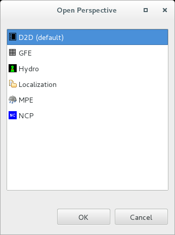
CAVE is the core visualization software for AWIPS, and it facilitates loading different suites of visualization software displays called perspectives:
D2D (Display in 2 Dimensions) - display multi-sensor data and issue short-fused warnings/advisories
GFE (Graphical Forecast Editor) - manage forecast grids and issue long-fused warnings/advisories
MPE (Multi-Sensor Precipitation Estimator) - manipulate precipitation estimates (advanced)
Hydro - interrogate river flooding and issue river flooding products
Localization - manage localization files
NCP (National Center Perspective) - for National Centers operations
Climate (not shown in image above) - used to issue climate products
CAVE is typically launched from the main Applications menu and "AWIPS Menu" submenu in the upper-left part of the Linux desktop on one of the monitors, but it can also be launched from a shell window using /awips2/cave/cave.sh with different command line arguments. For more information about CAVE command-line arguments see Chapter 25.10 of the System Managers Manual (available in the AWIPS2 VLab Community Library (requires standard NOAA LDAP password). Another useful reference page containing the CAVE - D2D User's Manual is the End Users AWIPS VLab page.
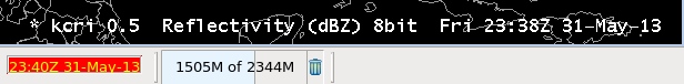
You can load multiple CAVEs per workstation, but each CAVE takes up a fixed amount of memory by default (WFOs 6GB for 20.3.2 and 8GB for builds after 21.4.1). While LX workstations typically have 32GB of memory available for WFOs, which theoretically could multiple CAVE sessions, the AWIPS Performance Group has recommended using no more than 2 CAVEs per workstation for heavy data intensive use. It is prudent to only load CAVEs and data when needed for workstation performance reasons. Typically CAVE is loaded full screen on each of the 27" monitors. The bottom of CAVE has a memory readout that you cave hover over with the mouse pointer to see how much of the available memory is being used:

The memory bar will turn red when you approach the limit for what CAVE has been allocated. Next to the memory bar there is a trash can icon that can be clicked to trigger "garbage collection" to free up memory. This will be covered more in the "Managing CAVE Displays and Memory Usage" WES video taken later.
CAVE is the visualization side of AWIPS, and it connects to the data management side of AWIPS called the Environmental Data EXchange (EDEX). At each office, CAVE has been configured to launch for a particular site (e.g. BOX for Boston) connected to an EDEX's Localization Server (to access localization files) and an Alert Server (to receive AWIPS alerts through the program AlertViz). In live operations, including service backup, you will always load CAVE as your local Site. When playing back data cases using the Weather Event Simulator 2 Bridge (WES-2 Bridge) machine, you will launch CAVE as different sites using multiple EDEXs. All the AWIPS localization files for CAVE and EDEX are managed through an intricate system of overrides with a specific hierarchy that is typically managed through the localization perspective or menus with override access in them:
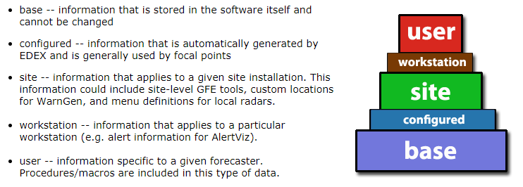
Overrides allow forecasters to copy a file the whole site can see and make a local copy to modify (e.g. user can override site, and site can override base). AWIPS localization is beyond the scope of this training, but it is good for forecasters to be aware of the concept of user and site overrides.
When launching CAVE with no optional arguments, it starts with the previously loaded perspective. Various icons and app-launchers can launch CAVE to start in a given perspective, like GFE. After launching CAVE, you will use the Open Perspective tool contained within the tool bar of CAVE (or the CAVE->Perspective menu) to change your perspective. This training will focus primarily on the D2D perspective.
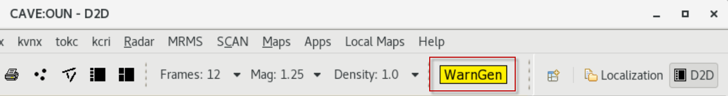
While there are no obvious separators between CAVE core features and the perspective loaded, you can think of the fundamental CAVE components as the CAVE menu, the perspective tabs bar (containing a tab for each perspective loaded) like tabs on a browser, and the CAVE clock on the bottom status bar. The rest of the menus, frame controls, and data displays are associated with the perspective loaded. The perspective tabs, WarnGen button, frame controls, etc. will wrap around to a new line if CAVE is shrunk laterally, so you always can't refer to elements in the toolbar being in a fixed location.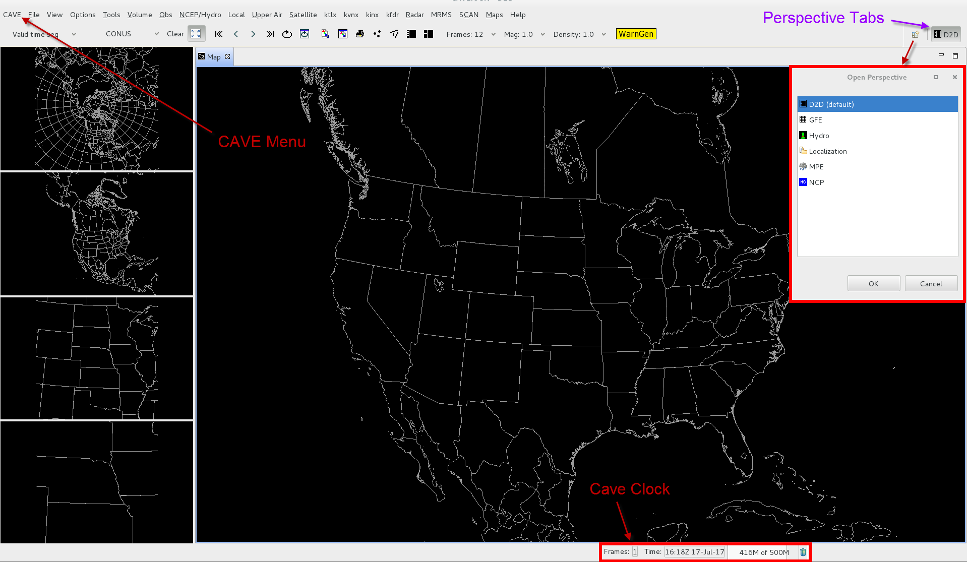
Perspective Display Pane and Map Editors
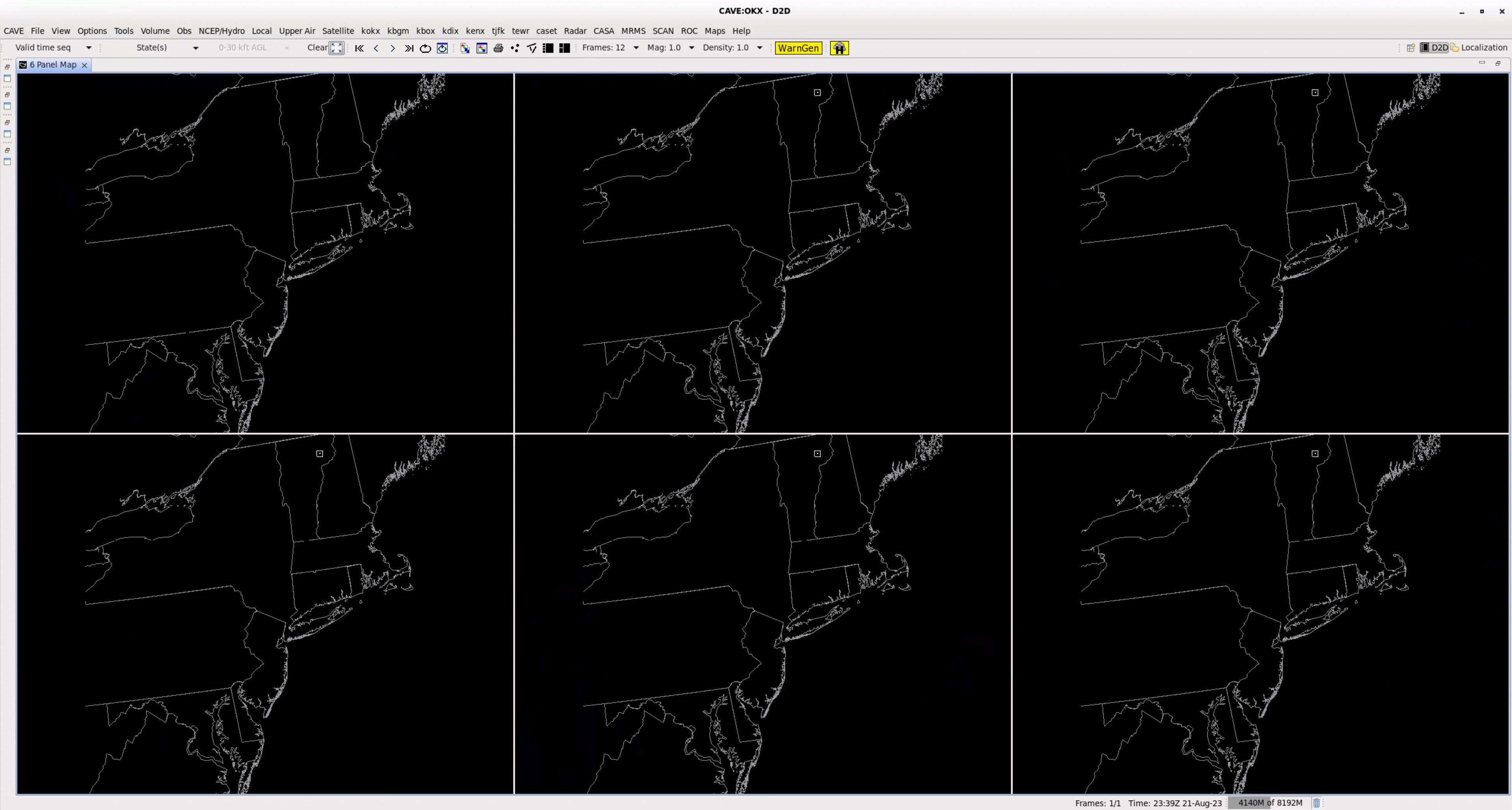
Each perspective display has at least one main display pane that is composed of different types of editors. Editors are atomic display elements in CAVE, and there can be map editors for viewing spatial data, an NsharpEditor for viewing Skew-T data, and even editors displaying lines of XML code you can modify. The default D2D perspective is unique in containing one map editor in the main pane and one map editor in each of the 4 side panes:
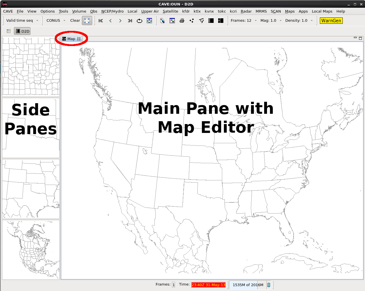
When you click on an editor to interact with it, any data or map loading requests from menus or loading procedure bundles will be completed in that editor. One important thing to know about map editors is that they function using a series of XML instructions for defining the product(s), map overlays, map projection, number of frames*, loop properties, etc. that can be saved in the perspective and edited using the localization perspective:
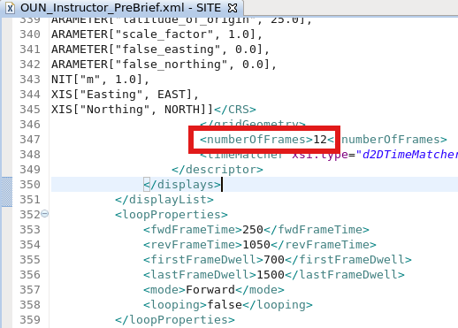
The XML representation is essentially a settings document that configure all aspects of the editor's display. This document can be saved in various ways, including procedures, display files, and perspective files which are described later.
*Note: If you are using an operational AWIPS 20.2.3 or later, you will see the frame number displayed with the total frame count at the bottom of the map editor window.

Most display manipulation in AWIPS is completed using simple perspective display menus and tools, but some of the newer innovations are having forecasters leverage the localization perspective. At this point it is important to think of your data and map loading/configuration in an editor as a series of instructions that are being translated into XML that you could modify in simple and complex ways.
Loading And Manipulating Additional Map Editors
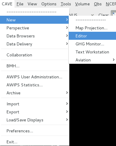
The main display pane is a unique area for editor manipulation in any perspective. Multiple editors can be loaded in the main pane by right clicking on the top of the main pane or by selecting New->Editor from the CAVE menu.
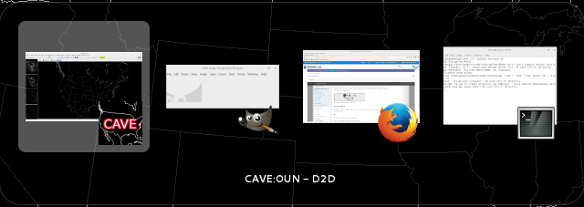
Each new editor is displayed separately like tabs in an Internet browser that can be accessed by selecting the tab name or using Ctrl + Page Up/Page Down to cycle through the tabs. The tab names in the main display panel can also be renamed using a right mouse click on the tab which is important when loading multiple tabs. Renaming the tab isn't just cosmetic; it changes the name of the bundle used to display the editor which you will see when you save display bundles into a procedure (covered later).

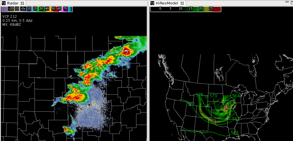
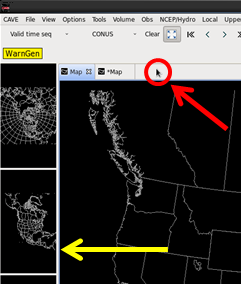
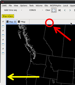
In addition to stacking multiple tabs next to each other, tabs can be moved around the main display and displayed simultaneously by dragging the tab and dropping it near the desired edge of the main display pane. When simultaneously displaying multiple tabs (see image below) each tab is independent of the others, so to interact with one tab to loop through or adjust the zoom, the user must first select the tab.
Map editors have icons in the upper-right for maximizing and minimizing the editor. When editors are minimized, they are pinned to the side of the CAVE with an icon that can restore them in the display.

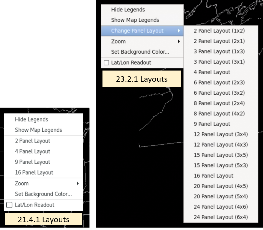
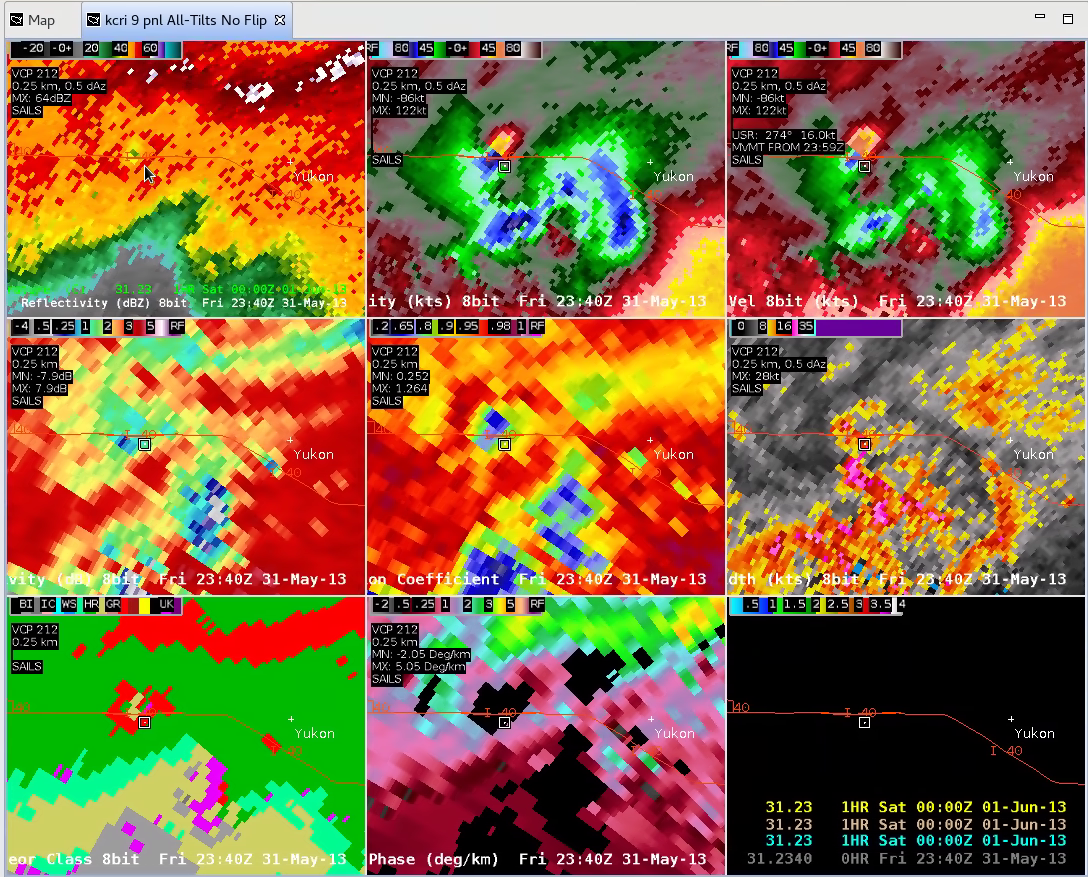
Map editors have independent controls, so if you zoom in and step through time for the data loaded in one editor, none of the other editors will respond to changes in zoom and looping in your one editor. To link multiple editors together an AWIPS focal point can modify the display bundle XMLs in the Localization Perspective (see this 9panel radar example used in RAC), or if you are configuring a map editor in the D2D perspective, a forecaster can simply use the Four Panel Layout option accessible with a right mouse click on the map editor.
Map editors are unique because they can be configured as a Single Panel Layout (default) or a variety of multi-panel layouts that are linked when zooming, sampling, and stepping through different times. The older AWIPS builds only supported single panel and four panels.
Side Display Panes
The D2D perspective is a unique perspective because it has multiple side panes that contain only one single editor that are used to view and store products. With a simple right click on the small pane you swap contents with the single active editor in the main pane ("swapping panes"). You cannot swap multiple editors at once into a single small pane. When data resides in the side panes, the right-click menu within the pane allows some minimal interaction such as looping and zooming on a subset of the data loaded. One major drawback of swapping panes is that every time data is swapped, the data is reloaded, which uses up memory and can take time for some types of data.
When the initial AWIPS software was developed, all panes were essentially limited to one editor, so the side pane layouts were essential in routine operations with D2D to rapidly swap in displays like other radars. Now that AWIPS has evolved to provide a configurable suite of editors and larger monitors have been implemented, more and more sites are migrating away from using the side panes in D2D to using highly configured perspective displays with groups of editors. If you want to maximize your editor display and shrink your side panes, you can move the vertical slider bar on the right side of the side panes far to the left, but the underlying eclipse software does not allow the side pane separator to be moved all the way to the left side of CAVE (limited to 10% of the width of the CAVE window). Fortunately there is a handy trick to effectively minimize the side panes by maximizing the main pane, either by 1) using the max/min buttons in the main pane window or by 2) double left clicking on the editor toolbar to toggle between max and min:
Unfortunately the maximized main pane with minimized side panes state can't be saved in the CAVE settings (i.e. Perspective Displays discussed later).
External Windows
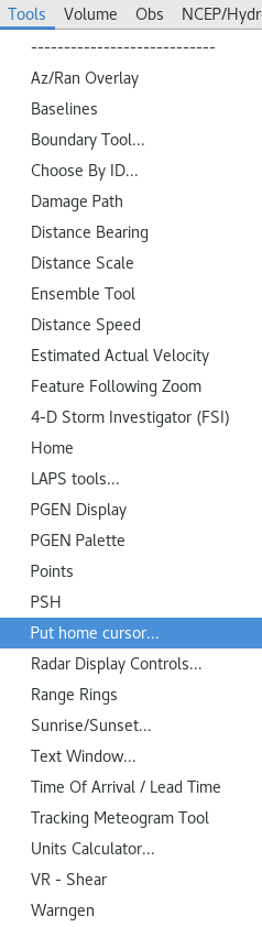
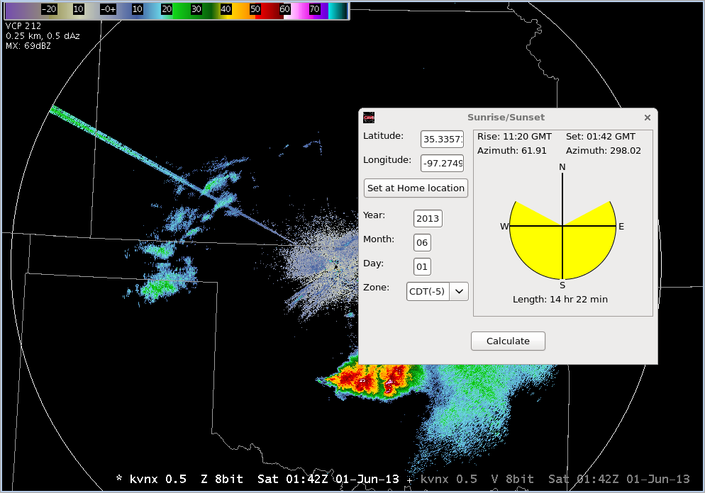
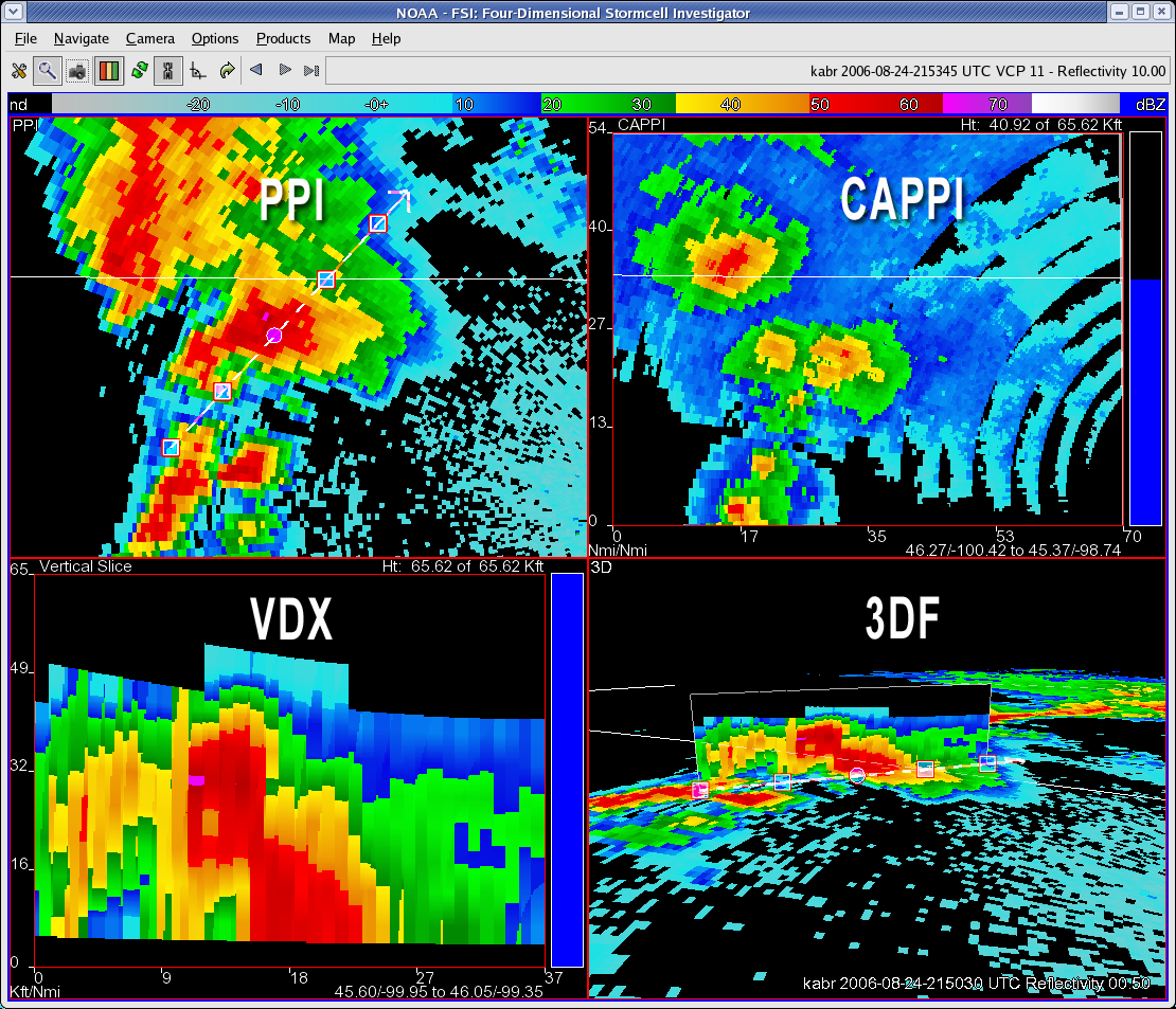
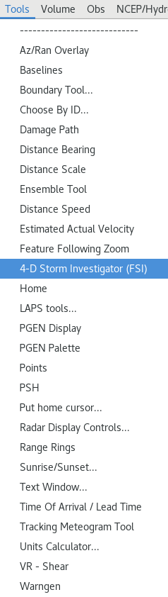
There are numerous tools across perspectives that use external windows that do not attach to CAVE like the Radar Display Controls loaded from the Tools menu:

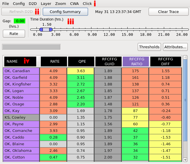
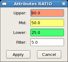
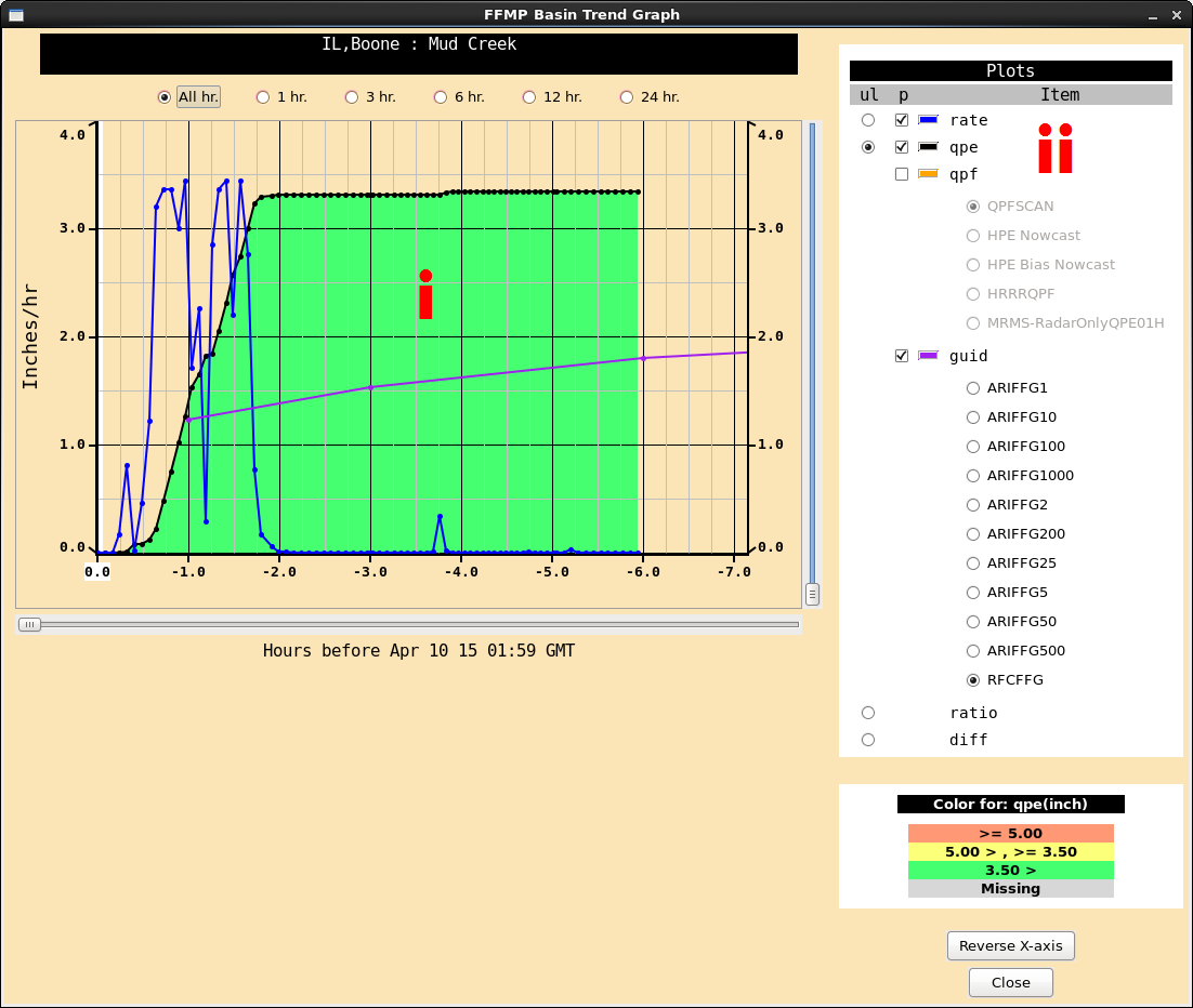
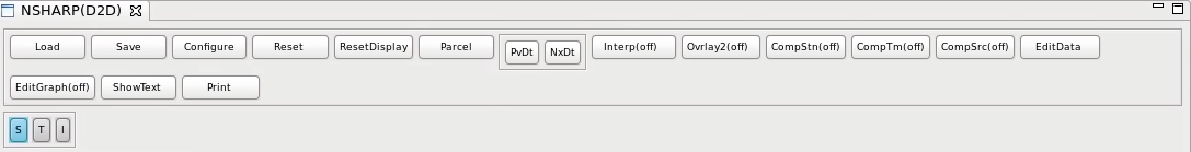
Some of these windows are simple Graphical User Interfaces (GUIs) that users will interact with to alter the appearance of data in the main display like the Radar Display Controls GUI. Some of these windows may be interactive tables or other displays that can control the appearance of the main display, but also allow for more detailed data analysis like the Flash Flood Monitoring and Prediction program. Other external windows are applications intended for performing data analysis in an environment separate from the main display like the Four-Dimensional Stormcell Investigator. Most external windows are effectively separated from the CAVE display, but a small subset of external windows can be attached to a CAVE editor (i.e. dock-able) like the NSHARP control buttons (discussed later).
Managing external windows in operations is crucial because smaller external windows can be easily misplaced on the display or get lost behind larger windows. One important technique for managing external windows is to cycle through windows by holding down the Alt button while repeatedly hitting the Tab button.
CAVE Menu Capabilities
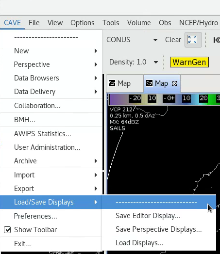
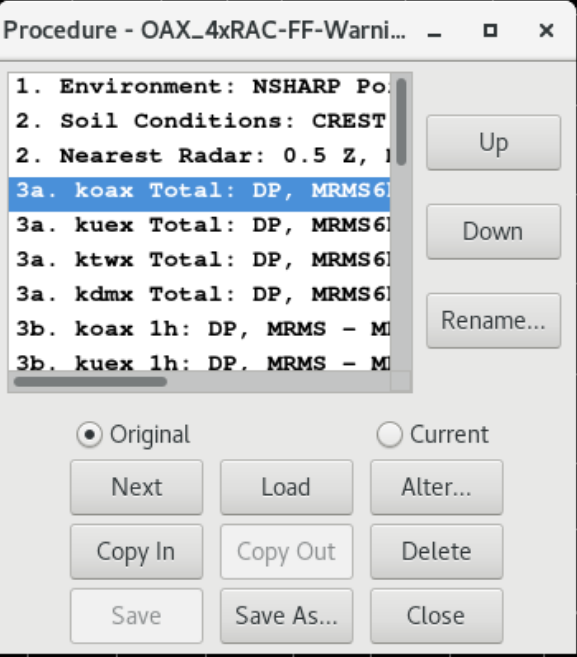
The CAVE menu contains a lot of different utilities for forecasters, focal points, and ITOs. One particularly important capability to point out for forecasters is the Load/Save Displays menu that allows the user to save an individual Editor Display or save all configured editors in the Perspective Display:
Perspective Displays are a powerful way to set up your workspace for different functions (e.g. aviation, severe weather, etc.). Below is a simple listing to identify the general functions of the menus:
New
Map Projection - create new Map Projection for a map editor
Editor - create a new Editor for a perspective's main display panel
GHG Monitor - launch the Graphical Hazards Generator (GHG) Monitor for issuing long-fused watches, warnings, and advisories
Text Workstation - launch a new Text Workstation (CAVE interacts with the last one loaded on a workstation)
Aviation - launch AvnFPS aviation software and its Configuration GUI
Perspective
D2D, GFE, Hydro, Localization, MPE, Other - launch a new perspective (same as CAVE open perspective button)
Data Browser
Product Browser - launch the Product Browser to directly load most data into a D2D editor rather than using perspective menus
Data Delivery
- manages special data subscription requests not on the Satellite Broadcast Network (e.g. NOMADS model data or MADIS observations)
Collaboration
- launch the Collaboration tool which will allow you to chat with other sites and share an editor display
BMH
- Broadcast Message Handler weather radio interface
AWIPS Statistics
- provides graphs of EDEX processing for ITOs to monitor AWIPS health
User Administration
- launches a window for ITO to control user privileges
Archive
Archive Case Creation - launch the Archive Case Creation tool which forecasters use to create an archived case from the 7-day rollover for use with WES-2 Bridge
Archive Retention - launch the Archive Retention tool which will allow the ITO to configure the data retained in the 7-day rollover
Both of the archive GUIs require special permissions that the ITO can configure using the AWIPS User Administration Window.
Import
Background, Image, GIS Data, BCD File, GeoTIFF, LPI File, SPI File, Displays - import images, GIS data, or a saved XML Display file into the current editor
Export
Image, Print Screen, KML, Editor Display - save current editor as an image, PDF, KML or save the raw XML code in an XML Editor Display
Perspective Displays - save the entire perspective configuration including all editors as an XML Perspective Display
Load/Save Displays
Save Editor Display, Save Perspective Displays, Load Displays - same as Import and Export Editor Displays or Perspective Displays
Preferences
- set forecaster preferences (Collaboration, GIS Viewer, Mouse, Rendering - font magnification, Tear-Off Menus)
- set ITO or Focal Point preferences (General, Localization, NCEP, Paths, Performance, Product Browser, PyDev, Text Workstation, XML)
- most forecasters primarily use the Mouse settings, so setting preferences is not common
Show Toolbar
- toggles the toolbar of the perspective loaded
Exit
- close CAVE (can also click x in upper-right CAVE window)
CAVE Fundamentals Summary
In summary, CAVE is used to load different software perspectives. A perspective contains unique tools for a particular forecast application and at least one main pane for assembling collections of atomic display XML instructions called editors. These distinctions become particularly important when saving and reloading perspective displays and editor displays. From the CAVE->Load/Save Displays menu you can save all the characteristics (data, maps, colors, etc.) in a particular editor using the Save Editor Display menu, and you can save all characteristics of all editors in the perspective using the Save Perspective Displays. While we will cover more on memory usage in the "Managing CAVE Displays and Memory Usage" WES exercise video, there are a few general guidelines worth pointing out in the CAVE fundamentals section:
General CAVE Guidelines
- load what you need as you go, not everything you could possibly use
- the amount of data loaded, including frame counts, matters, so pay attention to frame counts and scale of your displays
- trim frame counts back or reduce scales if you have memory or workstation performance issues
- pay extra attention to model derived parameters like CAPE and their data scale (more later)
- use multiple tabs instead of side panes to limit reloading data from a pane swap
- spread memory intensive applications across multiple CAVEs if you have problems
- if your memory bar on the bottom approaches the maximum available (8GB by default for WFOs operationally) it will turn red, and you can click the garbage icon to run garbage collection and free up some of the memory
Task: Transferring Screen Products Between the Main Display Pane and Side Panes
This task describes swapping display panes between the individual side panes and the main display pane, which allows multiple displays in the D2D perspective.
View Jobsheet
Task: Loading, Arranging, and Unloading Additional Map Editors
This task describes loading/unloading additional map editors, arranging map editors, and minimizing/maximizing editors.
View Jobsheet
Task: Saving Loading Editor and Perspective Display
This task describes loading/unloading additional map editors, arranging map editors, and minimizing/maximizing editors.
View Jobsheet
Map Backgrounds
Last modified date:
Jul 09, 2024
This lesson presents basic information on map overlays that can be loaded into a display panel and how the properties of those maps can be adjusted. There will be more detailed practice opportunities on this topic in WES Exercise #1 (CAVE Basics) on your office’s WES-2 Bridge machine.
Maps Menu
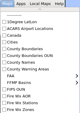
The Maps menu provides the AWIPS operator the ability to display numerous configurable map overlays in a single editor. Maps loaded from the Maps menu originate from the AWIPS mapsdata database. Typically the AWIPS focal point imports the maps into the mapdata database, so they can be simply loaded from the menu as simple overlays that have no time stamp. Additionally, forecasters can choose to manually import their own WGS84 non-projected latitude/longitude shapefiles as map overlays in D2D by using an application launched from the CAVE->Import->GIS Data menu. The import GIS Data approach can also be used to assign time to a map (for situations like burnscars) and can allow the user to filter the map displays and manage the properties of the attributes with finer granularity than when loaded from the Maps menu. Importing shapefiles is beyond the scope of this course, so we will focus on maps loaded from the Maps menu. If you would like to know more about importing GIS Data and are on the Internet, see this link.
Most maps, like cities and counties, do not significantly cover up underlying data, similar to graphic overlays like the Hail Index radar algorithm. The commonly-used HiRes Topo Image map is an example of an exception which is more like a radar reflectivity image that covers up underlying data. Knowing how to combine maps with adequate, but uncluttered and distinguishable, information is an important skill that can significantly enhance the speed and effectiveness of your data analysis during operations.
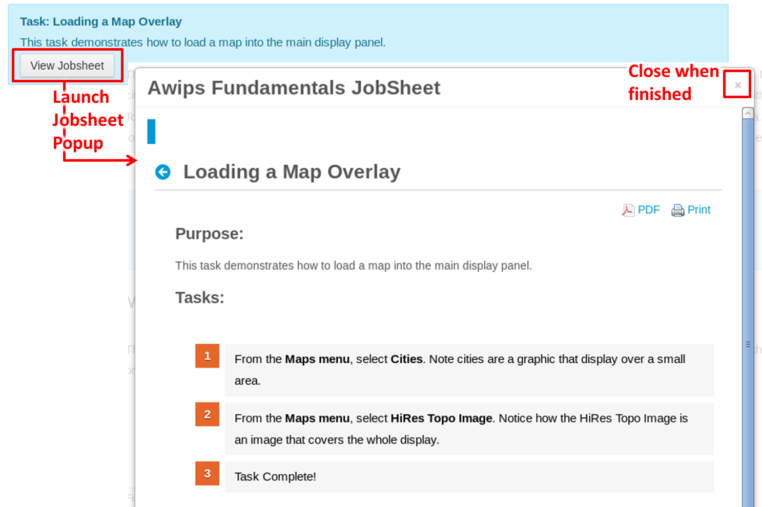
Task: Loading a Map Overlay
This task demonstrates how to load a map into the main display panel.
View Jobsheet
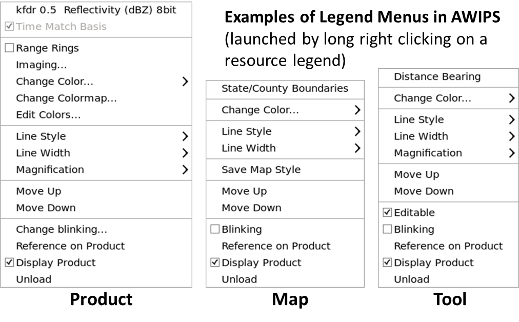
Map Legend vs. Product Legend
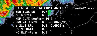
The lower-right part of the editor contains product legends and map legends that can be accessed through right clicks on the general editor background ("Show Map Legends" or "Show Product Legends") or by hitting the Enter key on the numeric keypad multiple times.
 (product legend)
 (map legend)
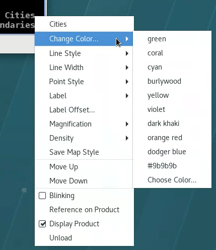
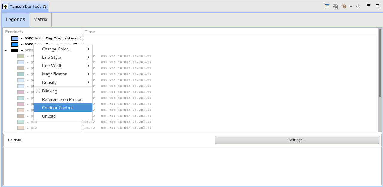
You can toggle the map legends on and off by left clicking on the mouse with the pointer over the name. You can also change map display characteristics such as color, line width, line style, etc. through a right-mouse click on the map legend name, and you can individually set the Density and Magnification settings for a product or overlay independently from all of the other products in your display:

Task: Unload a Map Overlay
This task will demonstrate how to unload a map that is currently loaded in the main display panel.
View Jobsheet
Editing Map Characteristics
Once the map legend is visible, use the context-sensitive menu (right click) to change a map’s characteristics. All configurable map traits are listed and discussed below.
Change Color...
Each map is displayed as one color (gray is the default). The color can be changed using the “Change Color...” option of the map legend menu. This option provides an interface where any RGB or HSB color can be applied to the selected map.
Line Style
Most maps, like county boundaries, are composed of line segments. The line style for a specific map can be changed under the “Line Style” option of the map legend menu. There are five possible line styles to chose from: Solid, Dashed, Dashed_Large, Dotted, or Dashed_Dotted. Solid is the default setting.

Line Width
Similar to line style, the line width of a map can be changed using the “Line Width” option. Four different line widths are available with the thinnest option being the default.

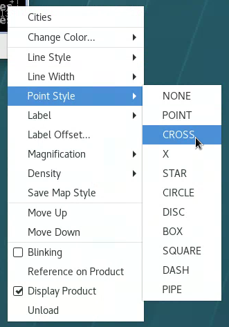
Point Style
For point-based maps like cities, the style of the point next to the label can be changed from a cross to a point or box.
Label and Label Offset...
For maps with multiple attributes like cities, different labels can be selected like NAME or POPULATION. The X and Y offset of the label from the point can also be controlled with the Label Offset... menu.

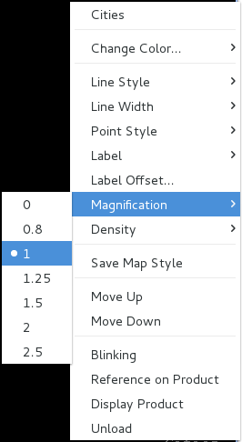
Magnification
For maps with text labels, the size of the labels can be changed by using the “Magnification” option of the map legend menu. There are seven different magnification settings available between 0 and 2.5 with 1 being the default value. Note that changes in the Mag setting in the D2D toolbar will apply to all maps, while changing the setting in a map’s menu only will apply to that map.
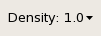
Density
For some maps like cities, the level of detail visible on different zoom levels can be adjusted. The number of markers or labels visible on a specific map is controlled under the “Density” option of the map legend menu. There are nine different Density settings available from 0 to Max, with 1 being a default baseline value and 0 not displaying anything. Like the Mag setting, the Density setting in the D2D toolbar will apply to all maps, while changing the setting in a map’s menu only will apply to that map.

Move Up/Down
Each map and product is a layer that can be moved up or down in the order in which they are displayed.

Task: Changing a Map’s Display Characteristics
This task demonstrates how to alter the default appearance of a map overlay by changing its display characteristics.
View Jobsheet
Editing Product Displays
Last modified date:
Jul 09, 2024
This lesson provides background information and step-by-step instructions on how to modify various product display characteristics.
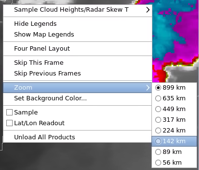
Changing the Zoom and Center
The center mouse wheel is the primary way to zoom in or out in an editor. CAVE also provides several different pre-defined zoom factors that you can utilize for those who don't have a mouse wheel or those who desire a fixed display, say for capturing sets of images over the same location. The zoom factors are defined by the map size (in km) in the display panel.
Task: Zooming In/Out of a Product View
This task will demonstrate the different ways to change the zoom factor in the main display panel.
View Jobsheet
Changing the center point
When viewing a product at one of the default scales (i.e. WFO), the center of the product will always be the center point of that default scale. You can change the map center by panning the image with a left mouse click and drag or by zooming in or out on the map. The location of the mouse pointer when you use the scroll wheel will zoom relative to that location.
Task: Panning a Zoomed-In Image in the Main Display Panel
This task will demonstrate how to pan the main display panel.
View Jobsheet
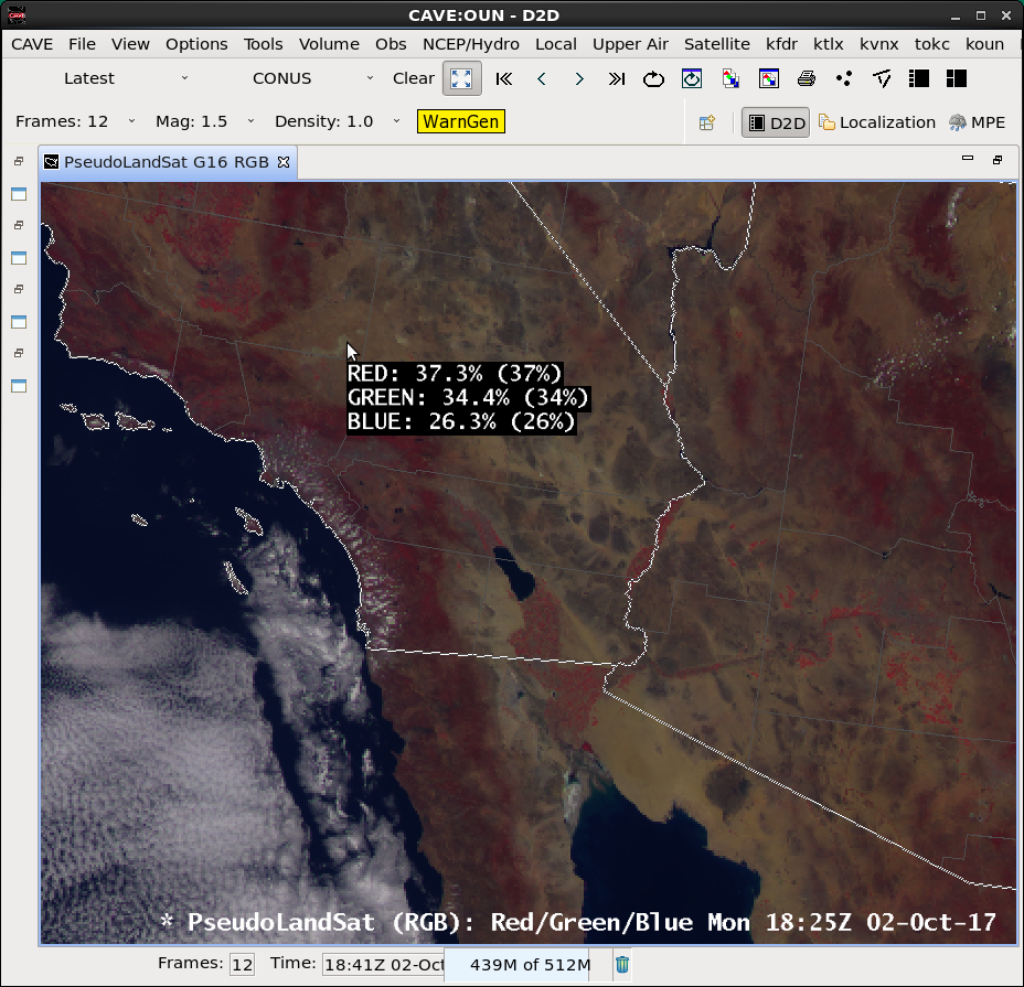
Sampling and Lat/Lon Readout
When products are loaded in an editor, data sampling and the latitude/longitude readout can be toggled on/off using the check box in the right click menu on the editor background (note this is different than right clicking on the product legend or map legend). Leaving sampling on can be distracting, and one best practice is to configure a long-left mouse click to sample on demand without having to use a menu selection. This will be covered later in the Mouse Settings page and WES Exercise 1 Cursor Sampling and Lat/Lon Readout video.
Changing the Image Color Table of an Image Product
Image products like radar and satellite data use color fills from a color table to indicate the data value for a particular location. Existing color tables can be applied to an image, or the color tables can be edited and saved as new files. Changing color tables manually is temporary unless you save them in a procedure or have your AWIPS focal point assign a new one to the menu loading.
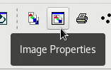
Switching color tables: The Image Properties GUI
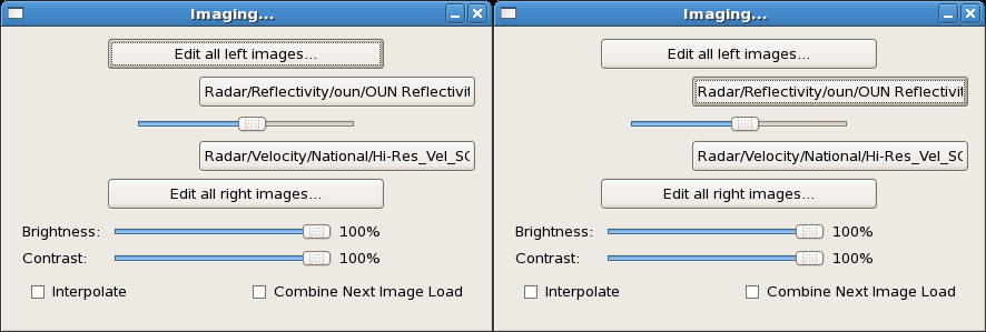
Most often, when you want to use a different color table, you just select a new one from the "Imaging" GUI launched by clicking the Image Properties icon on the toolbar or by using Ctrl + I keyboard shortcut. Note you can identify button functionality by hovering the mouse over the button in the toolbar. The Imaging GUI lists the color table for each image product loaded in the main display panel. Clicking on buttons reveals a pull-down menu for the color table options.
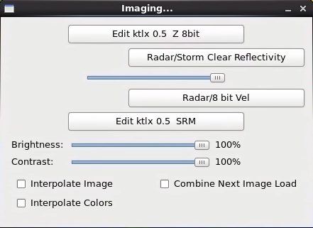
Another essential aspect of the Imaging GUI is the Brightness and Contrast controls. These are frequently used to reduce the brightness of displays so you can make other overlays more visible.
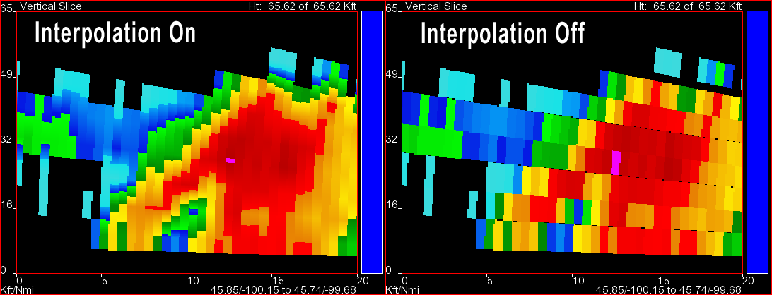
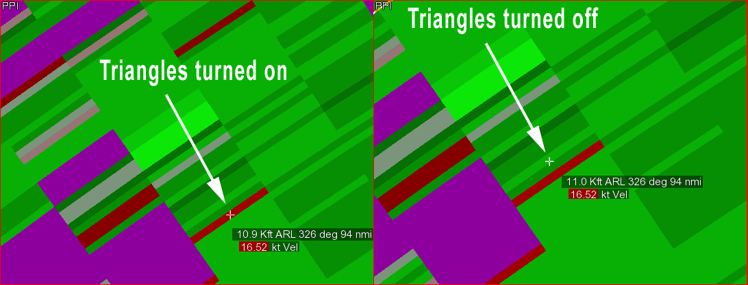
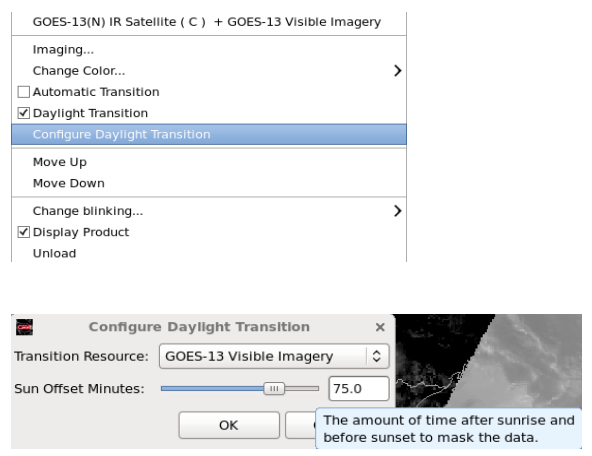
The Combined Next Image Load allows you to define paired products that can be faded back and forth. The Interpolate Image and Interpolate Colors will resample and smooth the data, particularly for grid data.
Task: Switching the Color Table for a Radar Image Product
This task demonstrates how to change the color table to another pre-existing color table for a radar image product.
View Jobsheet
Editing color tables: The Color Table Editor
The Color Table Editor allows you to modify the current color table. The GUI can be a little overwhelming at first because it provides the user with several options to change the color scale.
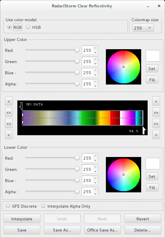
In the center of the GUI, the current color scale is shown with half-arrows on the top and bottom of the legend. Using the arrows, the operator specifies a range of data to define a color over. Depending on whether the image is a 4-bit or 8-bit/Super Res product, you can either fill that range of data values with a solid color or with a gradient of colors.
The colors used to fill or interpolate the range of values are determined from the two color panels in the GUI. These color selection panels give the user the option of using RGB (Red-Green-Blue) or HSB (Hue-Saturation-Brightness) color models to select a color. In addition to choosing colors, the transparency of the product can also be edited using the Alpha slider bar in the Color Table Editor.
When finished editing the color table, save the changes either to the old Color Table file or to a new file.
Task: Editing the Current Color Table
This task demonstrates how to make changes to the current color table using the Color Table Editor.
View Jobsheet
Blinking portions of a color table
Blinking the color table is a unique D2D perspective capability that can be useful at times to highlight important data. This can be useful for a warning forecaster who is color blind and who might have a difficult time distinguishing between two different colors used in a color table (even if the scale was specifically designed to mitigate this issue).
Task: Blinking a Range of Data Values
This task demonstrates how to select a range of values from an image product’s color table and make those colors blink.
View Jobsheet
Product Overlays
Last modified date:
Jul 09, 2024
This lesson provides instructions on loading multiple products into a single display, and it references tasks from previous lessons over loading and editing product displays.
Graphic Products vs. Image Products
When working in the D2D perspective within CAVE, it is important to understand the difference between image products and graphic products. In CAVE, graphics can be converted to images and images can be converted to graphics.
Graphic products
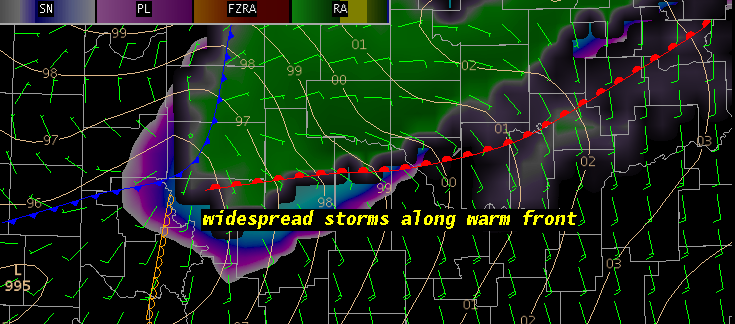
Graphic products are maps containing plotted or contoured data, soundings, or other plotted data. These products can be either observational data or model output products. Graphic products are beneficial for data analysis because multiple graphic products can be loaded into a single display panel and viewed concurrently over image products without masking the underlying data.
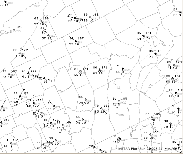
Graphic products contain less visual information than image products. Cursor sampling graphics only works for certain point measurements (e.g., surface observations). A single graphic product is displayed as one color, which can sometimes cause legibility issues. For instance, fields in a METAR station plot are all a single color, sometimes impeding interpretation. Further legibility issues can result from small font sizes or contour widths. Changing the panel Magnification and/or Density settings, or changing the product specific parameters (i.e., color, line width, etc.), can help mitigate some legibility issues with graphic product displays.
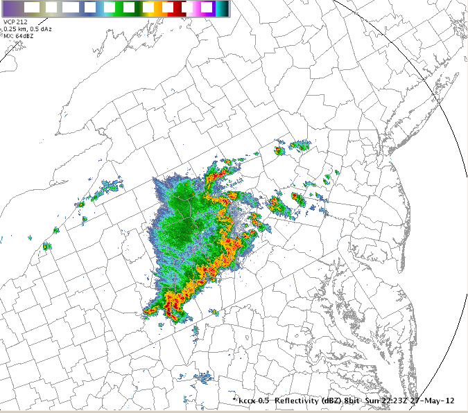
Image Products
Image products are continuous fields of data represented by color fills. The continuous color fill essentially creates a layer that can totally mask other layers of data underneath. The colors used in the color table can be changed or can be configured to blink, and the values can be sampled by right clicking on the background to select sampling or by configuring the mouse to sample using something like a long left click.
Pairing Combined Images and Product Stacking
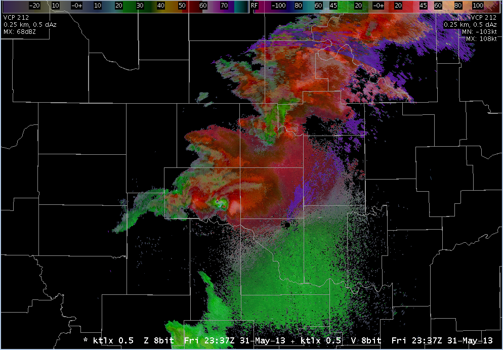
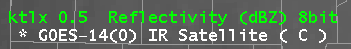
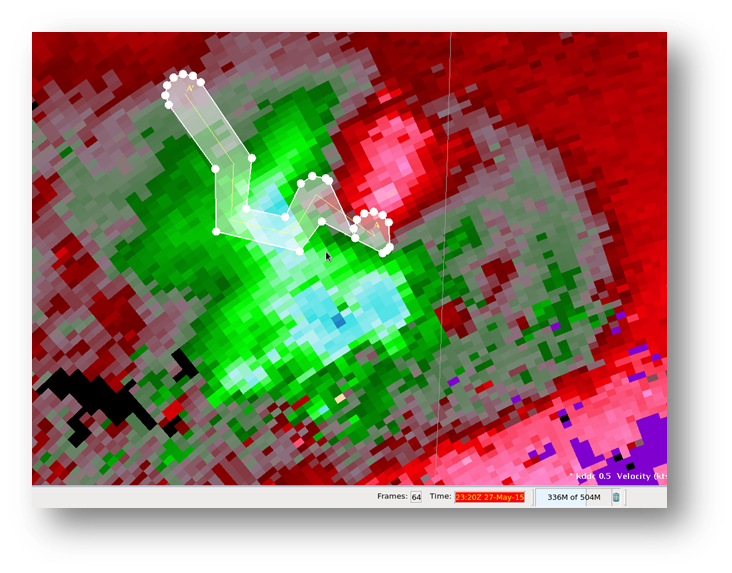
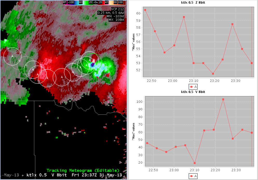
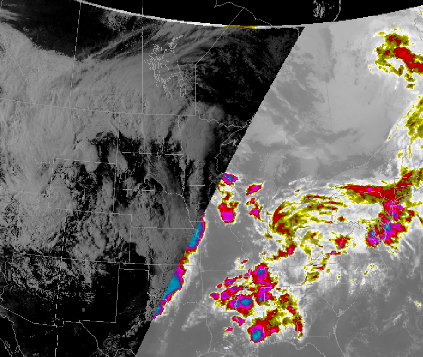
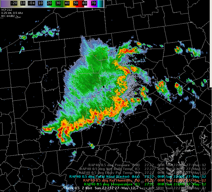
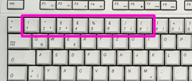
With the Combined Imaging button toggled on, when you load multiple images they are combined into one image where you can fade back and forth between the images using the +/- keys on the keypad or can toggle between images using the . on the keypad (with Num Lock on). The 0.5 Z/V product is a good example of this:
With the Combined Imaging button toggled off, when you load multiple images, they are stacked on top of each other. If they cover the same areas with their continuous color fills, then the top image typically will hide the data underneath unless the alpha channel for that color has been modified in the color table editor. Stacking can still be a viable way of loading multiple image products in an editor, but you will need to toggle the visibility of the image products by clicking on the product legends.
Task: Overlaying Model Image on Radar and Satellite
This task demonstrates how to load a radar image on a satellite image and add a model image.
View Jobsheet
Importance of Loading Order
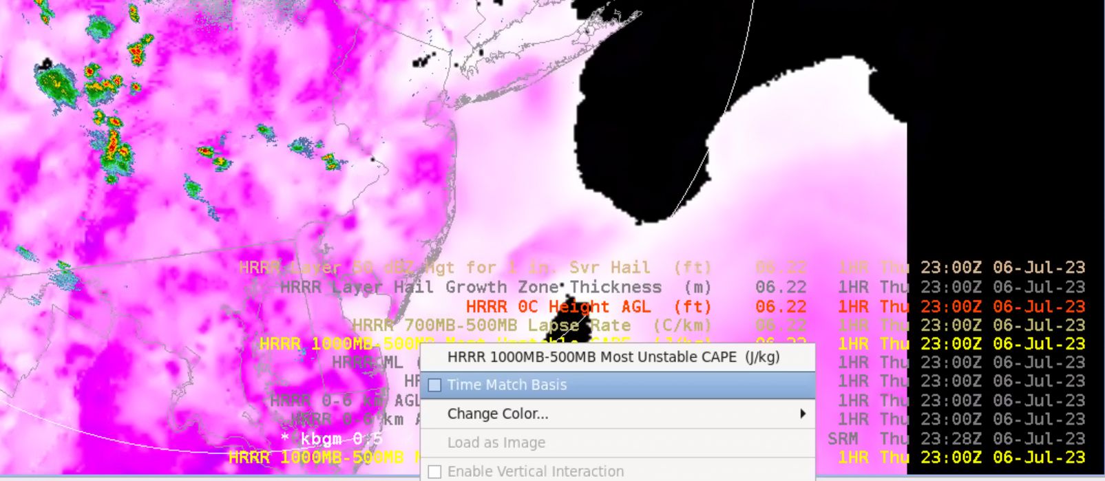
AWIPS operators commonly overlay graphics and image products on a single display panel. The sequential order of how products are loaded into the display panel is crucial to how those products update. The first product loaded into a display, by default, determines the Time Match Basis which is the frequency at which the frames in that display panel will update. This will put a * in the product legend to identify the Time Match Basis.
Once you have multiple products loaded, you can assign the Time Match Basis through a right-click menu on the product legend. It is important to consider the frequency of the products when choosing which product you want to drive the updating as the Time Match Basis.
For instance, if a METAR product is loaded first, then radar data, the hourly METAR data drives the frame contents. Changing the time match basis to the radar data will allow the 5-10 minute resolution radar data to drive the frame contents. Surface observation time matching is unique in that once you load an image over the initial graphic, the time match basis cannot be reassigned to the surface observation.
Task: Setting the Time Match Basis of a Product
This task demonstrates how to set the time match basis of a product in order to change which loaded set of data controls the update frequency of all data sets loaded in a current CAVE window.
View Jobsheet
Different Types of Graphic Product Overlays
Graphic products more subtly overlay image products because they typically do not contain the continuous color fills of an image product. Graphic products can vary significantly in their functionality and in their look and feel. In warning operations they generally fall into three categories: radar product overlays, Volume Browser product overlays, and other product overlays.
Radar Product Overlays
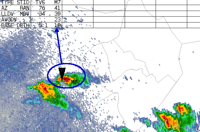
Numerous radar graphic products can be overlaid on radar image products. This includes such products as Storm Track Information (STI), Tornado Vortex Signature (TVS), and Meso Rapid Update (MRU). The number of pages in a particular table will be noted in the product legend at the bottom right of the screen by x/y, where x is the current page being viewed and y is the number of pages in the table. Multiple pages of radar graphic tables are cycled through by middle-mouse clicking on the product legend.
Task: Loading and Toggling Radar Graphic Overlay Products
This task demonstrates how to load and toggle a graphic product overlay into a frame after first loading an image product.
View Jobsheet
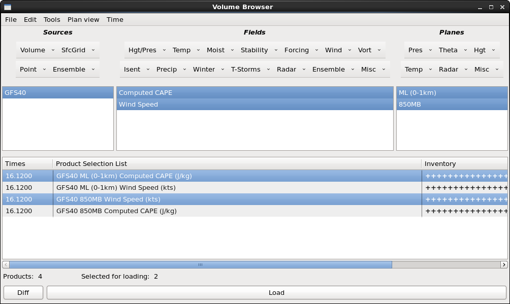
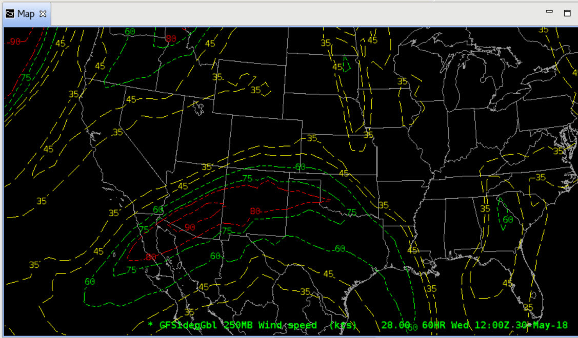
Volume Browser Product Overlays
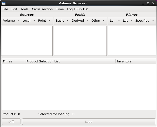
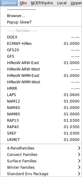
The Volume Browser is a unique tool in the D2D perspective that loads grid data from a user-selected Field (e.g. vorticity), Source (e.g. NAM12), and Plane (500MB pressure). You can load plan view (horizontal), cross sections, time height displays, variable versus height, sounding displays, and time series by selecting the type of display from the simple menus at the top of the Volume Browser window. While many grid data fields can be loaded from the D2D Volume menu Families, the Volume Browser allows you to load specific fields in your coordinate of choice (e.g. temperature, height, pressure, etc.). A detailed description of the Volume Browser and its usage falls outside the scope of this course. However, we will introduce some of the basics of the Volume Browser in the job sheets.
Task: Overlaying CAPE on a Base Reflectivity Product
This task will demonstrate how to use the Volume Browser to load a graphic overlay product (e.g., CAPE) in the same display panel as an image product (e.g., base reflectivity).
View Jobsheet
Other Product Overlays
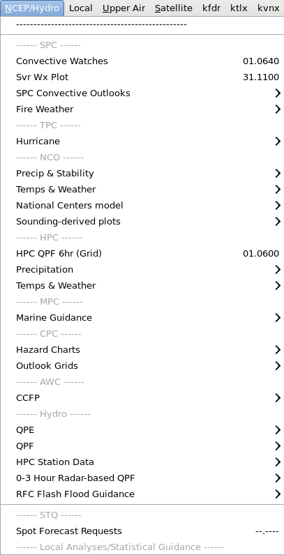
Other AWIPS graphic products such as METAR observations, warning polygons, etc. are useful to overlay on radar image products. These products are mostly located under the Obs or NCEP/Hydro menus in CAVE.
Task: Overlaying a Surface Plot on a Base Reflectivity Product
This task demonstrates how to load a graphic overlay (METAR surface observations) in a display panel with an image product (base reflectivity).
View Jobsheet
Import Export
Last modified date:
Jul 09, 2024
Printing the Contents of the Main Display Panel
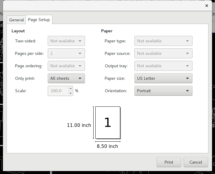
Making hard copies is a fairly straight-forward process in AWIPS. The Print GUI (File->Print or printer icon on D2D toolbar) gives you many of the basic options that you will see in any typical print dialog box: Portrait/Landscape, Scale, Copies, etc. 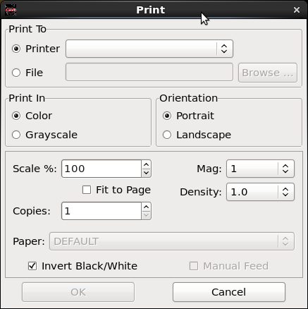
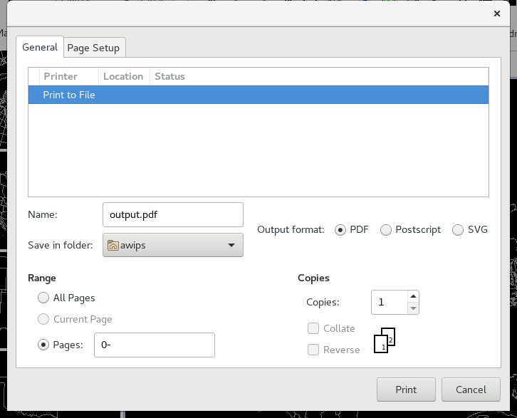
When you print hard copies, most often the “Invert Black/White” check box should be selected. This option prevents using excessive amounts of black ink. Situations where you will want to toggle this feature off include printing an image product that uses a primarily grayscale Color Table (such as Satellite Data) or image products with Color Tables that use white and black as particular data values that would somehow make interpreting the hard copy difficult. The other unique thing about the AWIPS print tool is that it gives you the capability to change the CAVE magnitude and density settings from the AWIPS printer dialog. If you select the File checkbox, then you can export the editor contents as a PDF.
Another way to print within AWIPS is using the Export option (CAVE->Export->Print Screen). This option contains basic print settings and will not let you toggle between black and white backgrounds, nor will it let you control the density and magnitude in CAVE.
Task: Printing the Contents of the Main Display Panel
This task demonstrates how to make a hard copy of the main display panel contents.
View Jobsheet
Exporting Screen Captures from AWIPS as an Image
Making images or animated GIFs is very easy in AWIPS using the capture utility under CAVE->Export->Image. To make readable images you should pay attention to image size and label readability. Resize your CAVE display so the editor with the data is the the desired pixel size. Second, increase the magnification of the product legend (right click on product legend or adjust Mag in the toolbar), so the fonts are clearly readable for the text legends. If you have multiple frames loaded you specify to create a separate image for each, and you can also create an animated gif. AWIPS has some video capture capability with the FFmpeg application (see the 17.2.1 tab on the AWIPS Builds page and the 17.2.1 Informational Overview for more details).
Task: Creating a Screen Capture of the Main Display Panel
This task demonstrates how to make an image file or a series of image files of the main display panel contents.
View Jobsheet
Text Products
Last modified date:
Jul 09, 2024
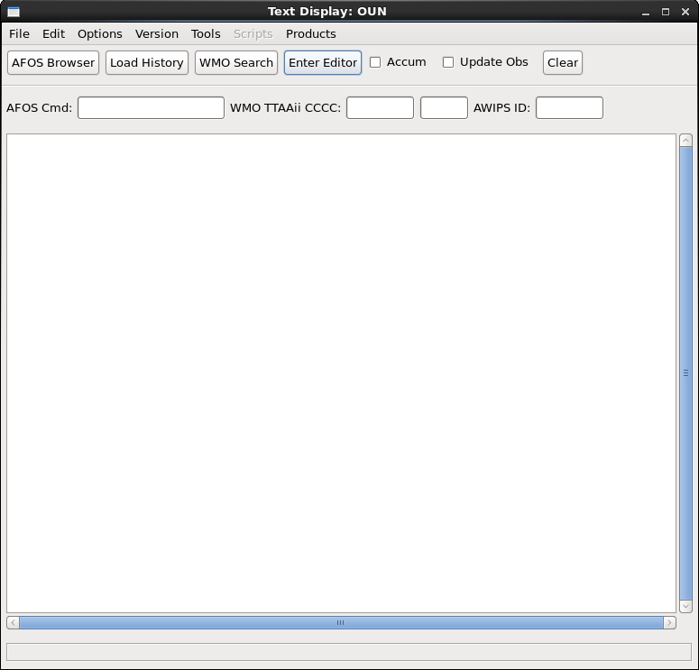
This lesson provides instructions on how to use AWIPS text windows to display a variety of text products commonly referenced by three-letter text product IDs or by 9-character Automation of Field Service Operations and Services (AFOS) Product Inventory List (PIL) references. For a comprehensive list of 3-letter text product IDs, see this NWS Weather Forecast Office Product Listing. For a detailed listing of AFOS PILs for most NWS offices, see this version of the afos2awips file (web content, text file). These text products can be alphanumeric radar products generated by the WSR-88D or any of the text products generated by a WFO that are currently in the local database. On AWIPS, text products are viewed using the Text Monitor which can be launched from the CAVE->New->Text Workstation menu.
Displaying Alphanumeric RPG Products
While most products generated by the WSR-88D Radar Product Generator (RPG) can be displayed as graphical or image products in the D2D perspective, some products contain text information designed for display in a text window. These products are often referred to as Alphanumeric RPG Products. Some of these products are simply text products (e.g., Free Text Message) while others contain text information embedded within a graphic product and can only be displayed in a text window (e.g., adaptable parameters of the Tornado Vortex Signature).
Here is a list of the different alphanumeric RPG products you can view in a text window (including the three letter identifier for that product):
Alphanumeric RPG Products That Are Viewable in a Text Window
| Product Name |
Three-Letter Identifier |
| Free Text Message |
FTM |
| Hail Index |
HAI |
| Mesocyclone |
MES |
| One Hour Precipitation |
OHP |
| One Hour Snow Depth |
OSD |
| One Hour Snow Water Equivalent |
OSW |
| Product List |
PTL |
| Radar Coded Message |
RCM |
| Storm Structure |
SST |
| Storm Total Precipitation |
STP |
| Storm Total Snow Depth |
SSD |
| Storm Total Snow Water Equivalent |
SSW |
| Storm Track Information |
STI |
| Supplemental Precipitation Data |
SPD |
| Three Hour Precipitation |
THP |
| Tornado Vortex Signature |
TVS |
| User Alert Message |
USM |
| User Selectable Snow Depth |
USD |
| User Selectable Snow Water Equivalent |
USW |
| VAD Wind Profile |
VWP |
The steps for displaying these products are shown in the following task that covers how to view a VWP product.
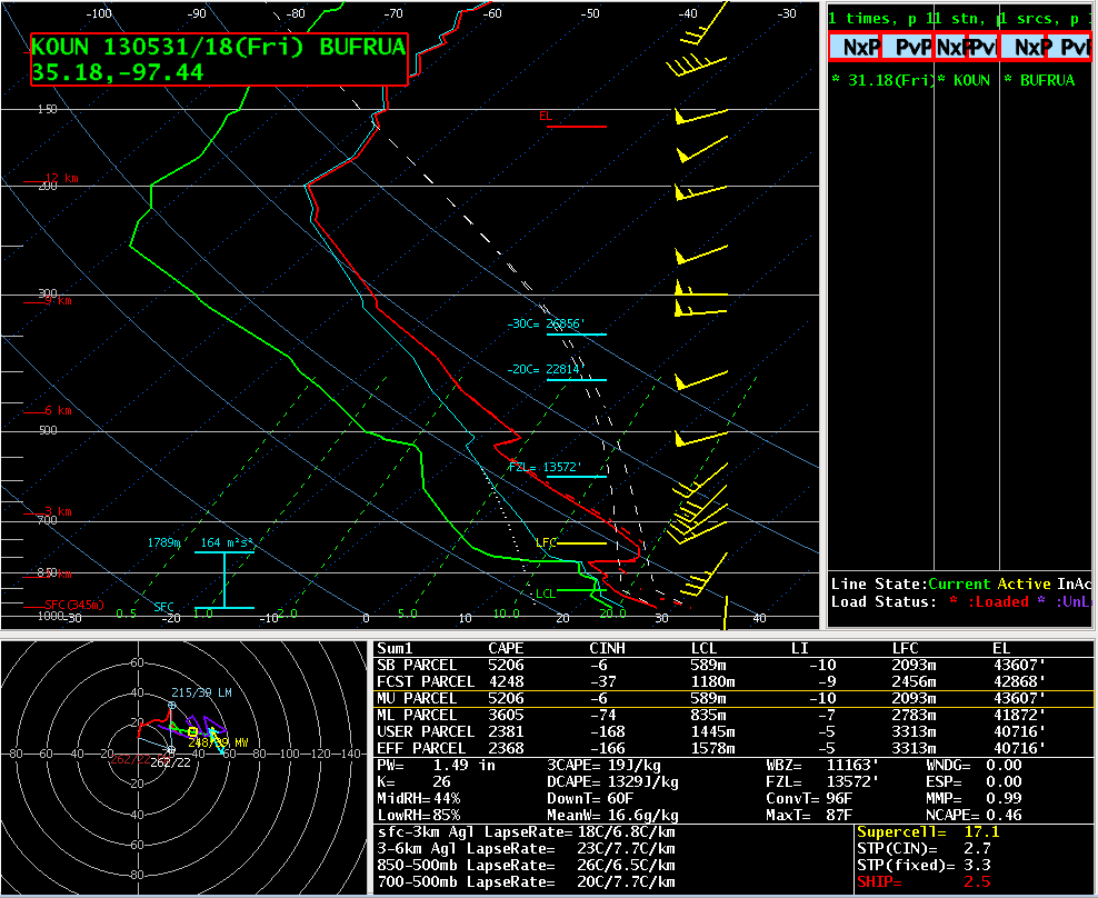
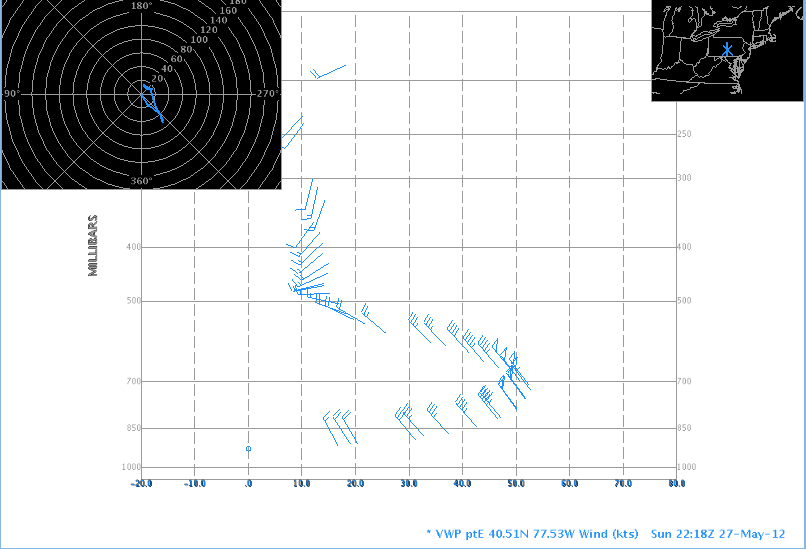
Task: Loading the Alphanumeric Information for a VWP Product
This task demonstrates how to use a text window to access the attribute and adaptable parameter information embedded within a VWP product.
View Jobsheet
Displaying Office Text Products
In addition to RPG alphanumeric products, the AWIPS text window can display any text product currently in the AWIPS database. These products may be issued by your local office or by neighboring offices which are pertinent to your operations.
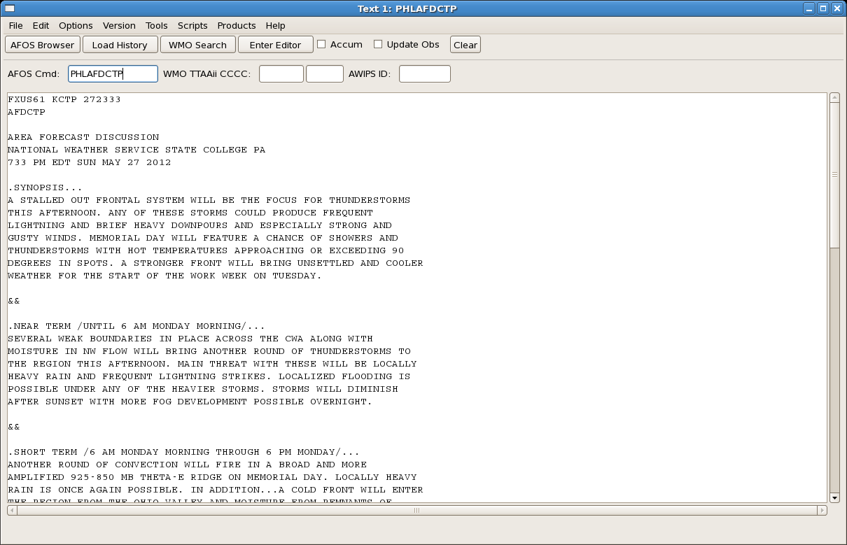
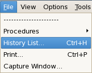
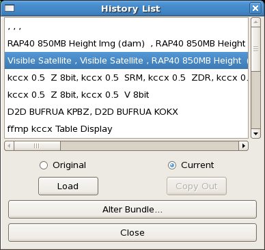
There are several ways to access these products in a text window (see NWS Weather Forecast Office Product Listing for product listing). Like RPG alphanumeric products, the nine-letter ID (see AFOS PILs) for a product in the “AFOS Cmd:” entry field retrieves all instances of that product from the database. Alternatively, the AFOS Browser provides a GUI used to select the Node, Category, and Designator from menus that construct the nine-letter ID for a text product. The AFOS Browser is particularly useful for loading less common products. Lastly, you can use the Load History to open text products that have been viewed previously on that AWIPS workstation.
Task: Using the AFOS Browser to Load an Area Forecast Discussion
This task demonstrates the steps for using the AFOS Browser to view an Area Forecast Discussion (AFD) from your local office AWIPS database.
View Jobsheet
Mouse Settings
Last modified date:
Jul 09, 2024
This lesson provides a brief description of the mouse controls and user-configurable mouse settings, so you can adjust your own mouse settings. While many of the mouse settings are not routinely changed, there are some mouse settings that are commonly used. One WDTD recommended change to the AWIPS defaults is to enable image sampling with a long left click. This allows you to sample and roam on demand which is a critical skill in warning decision making.
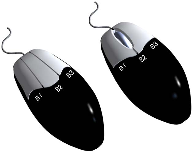
Mouse Shortcuts Tables
The three-button mouse performs a number of actions, depending on where in the CAVE window the mouse pointer is located. Here, each button is referred to by number: Button 1 (B1), Button 2 (B2), and Button 3 (B3). If your workstation has a two-button mouse with a clickable scroll wheel, all references to Button 2 in this lesson refer to the clickable scroll wheel.
The tables below detail the different functions for each mouse button for the default AWIPS mouse settings.
Mouse Functions for B1 (Left Mouse Button)
| Function |
Mouse |
| Open pull-down menus in the menu bar |
Click B1 |
| Create tear-away menus by selecting the dashed line in the pull-down menu |
Click B1 |
| Make menu selection in menu |
Click B1 |
| Activate menu buttons in toolbar |
Click B1 |
| Toggle product on/off in product legend in main map editor |
Click B1 |
| Drag slider to desired setting on a slider bar in a dialog box |
Press and Hold B1 |
| Moving any of the following items in a main map editor and any other map editor: Point, Baseline, Distance Speed, WarnGen vertex, and Select Alert Area |
Press and Hold B1 |
| Bring a window to front |
Click B1 |
| Move a window or dialog box |
Press and Hold B1, then Drag Mouse |
| Pan across large display (Pan feature must be activated) |
Press and Hold B1, then Drag Mouse |
Mouse Functions for B2 (Center Mouse Button or Clickable Scroll Wheel)
| Function |
Mouse |
| Zoom in (Pan feature must be activated) |
Scroll Forward, Middle Click |
| Zoom out |
Scroll Back |
| Pan across large display (Pan feature must be activated) |
Press and Hold B2, then Drag Mouse |
| Toggle on/off Editability of tool in Tool Legend of main map editor |
Click B2 |
| Insert/Delete vertices when editing on lines/vertices of warning box |
Click B2 |
Mouse Functions for B3 (Right Mouse Button)
| Function |
Mouse Action |
| Swap small display pane with the large display pane containing the main map editor |
Click B3 |
| Launch CAVE window options in title bar of CAVE display or dialog box |
Click B3 |
| Toggle all product legends within selected map editor (small or large display pane) |
Click B3 |
| Launch color table by selecting product in Product Legend of main map editor |
Click B3 |
| Open respective pop-up menu on legend or over displayed products in any map editor/pane |
Press and Hold B3 |
| Open pop-up menu on product name listed under Product Selection List in Volume Browser |
Press and Hold B3 |
| Toggle Alert Cells in radar alert area |
Click B3 |
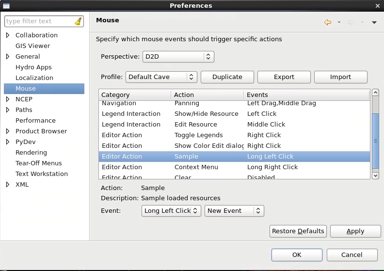
Configuration of Mouse Buttons
In AWIPS, you can set the mouse settings to your own personal preference. They are stored on the EDEX server under your username and are available on any workstation into which you log in. However, there are two issues with using modified mouse settings. One is your individual settings are not available to another user. If workstations are shared during active weather, you need to be familiar with the mouse settings of your collaborators. The default settings are always available. The second issue is the mouse setting configurations could possibly be reset after a server software upgrade if the settings were not preserved prior to the upgrade and migrated after the upgrade.
For the D2D perspective, there are two different mouse profiles available: Default Cave and AWIPS 1 D2D. The table shown here lists the default mouse settings for both Default Cave and AWIPS 1 D2D. Note that it is possible to overwrite the default settings. Therefore, this listing will help to restore the actual default settings.
Default Mouse Settings
| Category |
Action |
Default Cave Event |
AWIPS 1 D2D Event |
| Navigation |
Zoom Out |
Scroll Back |
Left Click |
| Navigation |
Zoom In |
Scroll Forward, Middle Click |
Middle Click |
| Navigation |
Panning |
Left Drag, Middle Drag |
Middle Drag |
| Legend Interaction |
Show/Hide Resource |
Left Click |
Left Click |
| Legend Interaction |
Edit Resource |
Middle Click |
Middle Click |
| Editor Action |
Toggle Legends |
Right Click |
Right Click |
| Editor Action |
Show Color Edit dialog |
Right Click |
Right Click |
| Editor Action |
Sample |
Disabled |
Long Left Click |
| Editor Action |
Context Menu |
Long Right Click |
Long Right Click |
| Editor Action |
Clear |
Disabled |
Disabled |
Note that you can assign multiple actions, like panning and zooming, to a single mouse control. Sometimes, these will not conflict, like setting left click to zoom out and show/hide resource (default). Sometimes these will conflict, like when left click is assigned to show/hide resource and sampling. In this instance, the sampling overrules the show/hide resource, so you can’t toggle the products with the left mouse button. If you encounter a conflict, try assigning one of the mouse controls to a different action (e.g., long left click for sampling and left click for show/hide resource).
You can also have conflict with different actions in one mouse button, like left-click pan and long left-click mouse sampling (i.e., Cave Defaults modified with sampling turned on). This particular conflict can be mitigated by disabling the pan button in the CAVE toolbar or by rapidly double clicking and holding on the second click.
Alerts and Data Monitoring
Last modified date:
Jul 09, 2024
This lesson provides basic user instruction on the AWIPS alert management application called AlertViz.
---------------------------------------
AlertViz Overview
The main interface for AlertViz is a thin window outside of CAVE containing a row of status icons (related to FFMP, FOG, SafeSeas, SCAN and SNOW alerts) and general AWIPS alert text log controls. AlertViz provides different alerts through the use of pop-ups, colors, and sounds. Your ITO can configure AlertViz to alert in different ways to tailor some of the notifications, but AWIPS by nature generates a lot of alerts that you will need to know how to manage.

Note: In live operations AlertViz is started when the user logs in, and it must be running for CAVE to launch.
Task: Move and Adjust Width of AlertViz
This task will demonstrate how to move the AlertViz bar in your window and how to adjust the width of the AlertViz bar.
View Jobsheet
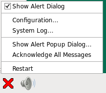
Hiding the AlertViz Dialog Box
You can hide and show the AlertViz bar by toggling on/off the “Show Alert Dialog” option in a menu that appears by right-clicking on the AlertViz icon in the task bar on your machine's desktop. While hiding the AlertViz bar can reduce the clutter on your screen, there is one important consequence. When hidden, you cannot see certain text-only responses or alerts (i.e., alerts that have a low system priority). Alerts with higher priorities will still trigger pop-ups and sounds that the forecaster will see.
Text Section Log
The Text Section Log in AlertViz allows the user to obtain more detailed information on a message and to filter messages by category. A list of AlertViz messages can be launched from the AlertViz bar. The window that contains these messages provides the option to show more detail about a message in a split-screen format.
Task: Launch Text Section Log and Display Detailed View
This task will demonstrate how to launch the Text Section Log and show the details of a message within the log.
View Jobsheet
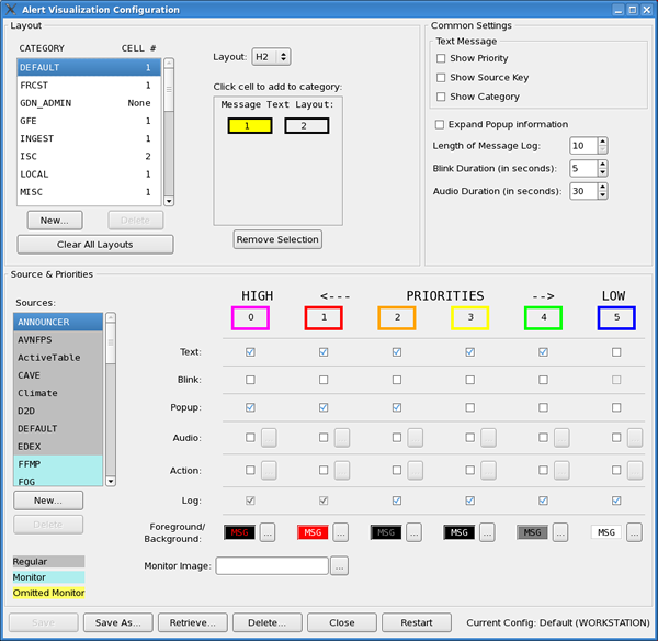
Alert Visualization Configuration GUI
The Alert Visualization Configuration GUI allows you to working with your ITO to configure message alerts to reduce notification distractions. The image on the next page shows what the configuration GUI looks like. Within this GUI, you can create and save different configuration files. Some of the properties that can be adjusted include the following:
- Message text layout
- Text message settings, such as the ability to show message priority and adjusting the blink/audio durations
- Visual/audio settings for each of the different priorities from High (Priority 0) to Low (Priority 5) for different sources (CAVE, EDEX, FFMP, etc.)
The Alert Visualization Configuration GUI is launched from the menu that appears by right-clicking on the AlertViz icon in the task bar on your machine. In this menu, you would select the “Configuration...” option and press the left-mouse button. See your ITO or local AWIPS Focal Point before changing any of your alert settings because you don't want to miss a critical alert!
Using the AWIPS Data Monitor
This lesson provides instructions on how to assess data outages. Because the AWIPS monitoring capability is not integrated in the WES-2 Bridge, this lesson requires a live AWIPS.
---------------------------------------
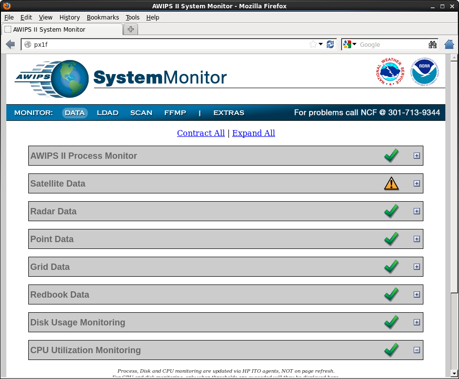 The AWIPS Data Monitor is part of the AWIPS System Monitor, which provides a status of the AWIPS Data (Radar, Point, Grid, Satellite, Local, Graphic, and Disk Usage) and the data ingest processes. The page is composed of collapsible tables with a data label and a corresponding state value. The state is characterized by one of four symbols: a green check mark, a red circle with a white “X”, a blue question mark, and a yellow triangle with a black exclamation point. Each one of these has a specific meaning.
- A green check mark indicates that data are being received in a complete and timely manner.
- A yellow triangle with a black exclamation point indicates that data are somewhat late (i.e., more than 20 minutes old) or the data disks are running at a somewhat high level.
- A red circle with a white “X” indicates that data are very late (i.e., more than 40 minutes old) and/or very incomplete.
- A blue question mark indicates that no files are present in the data storage for that data set (i.e., perhaps a dedicated radar is down for maintenance for an extended period of time).
Clicking on the plus sign (“+”) in the Data Monitor page provides a more detailed listing of products within each data type, as well as the respective state of each data product. If a symbol other than a green check mark appears in the status column of a particular data set, it is important to click on the plus sign to see which product(s) may have problems.
NOTE: It is important to note that a yellow triangle denotes a problem that is logged by the Network Control Facility (NCF), but not necessarily known by NCF controllers. However, a red circle denotes a problem that would be visible on a NCF controllers monitor. It is important to communicate any system problems with the NCF using local guidelines.
Note: The AWIPS Data Monitor is only available on a live AWIPS workstation.
Task: Loading and Using the AWIPS Data Monitor
This task demonstrates how to load the AWIPS System Monitor and how to navigate to the detailed listing in the AWIPS Data Monitor.
View Jobsheet
 This reference provides an introduction to the fundamental AWIPS functionality supporting convective warning analysis and decision making. It is composed of a series of web pages with embedded job sheets used to practice fundamental skills on a live AWIPS or WES-2 Bridge. This training mostly focuses on CAVE basics and the D2D perspective (not GFE, AvnFPS, etc.), and it is followed by separate WES-2 Bridge exercise videos that step through using the tools with an archived dataset. Following review of the VLab web pages, practicing with the embedded job sheets, and practicing along with the WES-2 Bridge exercise videos, proficiency is assessed with a locally proctored AWIPS proficiency exam. Most of the content in this reference does not change from build to build, but some of the differences between the live AWIPS builds and some of the older AWIPS in the WES-2 Bridge versions are listed below. The 17.3.1 WES-2 Bridge local machines are being replaced by a 19.3.4 WES-2 Bridge that is available through a WFOCluster machine in the cloud that the local facilitator organizes.


 (
(


