Purpose:
This jobsheet reviews the NSEA Digital Cursor Readouts and contrasts this with the related Standard Environmental Packages (30-40min).
Tasks:
Sections
-
-
-
-
-
-
-
- Overview: Now that the Near-Storm Environmental Awareness (NSEA) Digital Cursor Readouts are baselined in 21.4.1, there are two primary types of environmental sampling available in the Volume menu:

The Standard Env Packages map out base state environment fields like temperature, relative-humidity, wind, etc. to their 3D location associated with height-based radar fields, whereas the NSEA Digital Cursor Readouts display any derived parameters to any products loaded in 2D space and are not interpolated to a particular height.
The NSEA Digital Cursor Readouts was developed to facilitate increased situation awareness for radar operators and meso-analysts by displaying critical parameters about the mesoscale environment superimposed on radar data. When sampled, the readouts are displayed for select parameters without needing to load those elements as images, as AWIPS typically requires. The NSEA Digital Cursor Readout was evaluated at the Operations Proving Ground and consensus was that it was intuitive, easy to use, and extremely valuable in warning decision making and short-term forecasting.
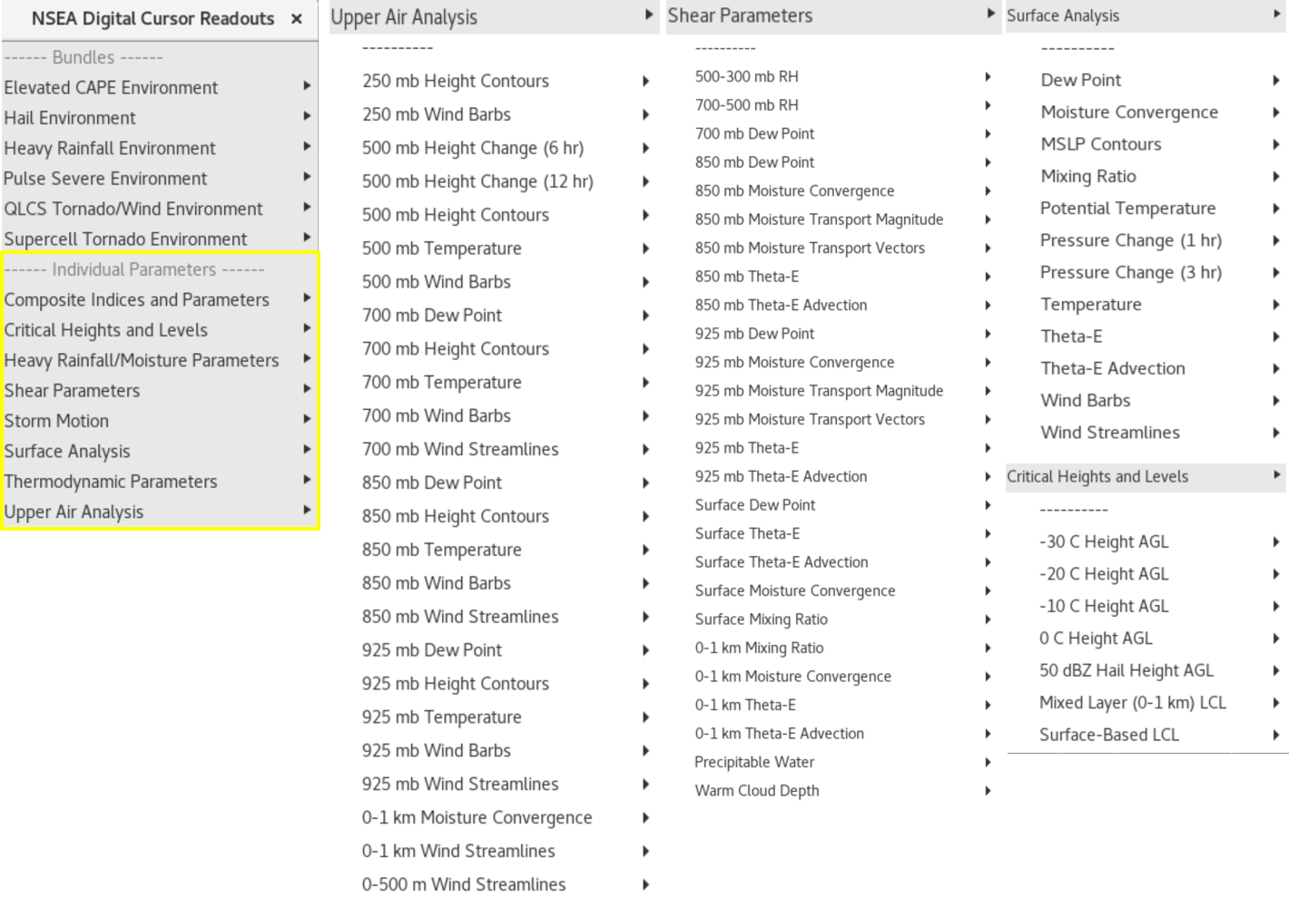
The NSEA Digital Cursor Readouts effectively map out most severe weather and flash flood parameters calculated in the Volume Browser into an easy-to-find set of menus. You can choose to overlay one individual parameter on whatever product you have loaded, or you utilize the bundles which have groups of parameters organized by environment applications like hail or heavy rainfall.
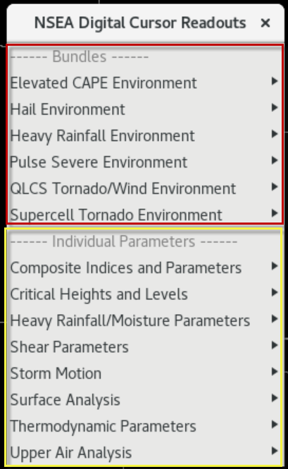
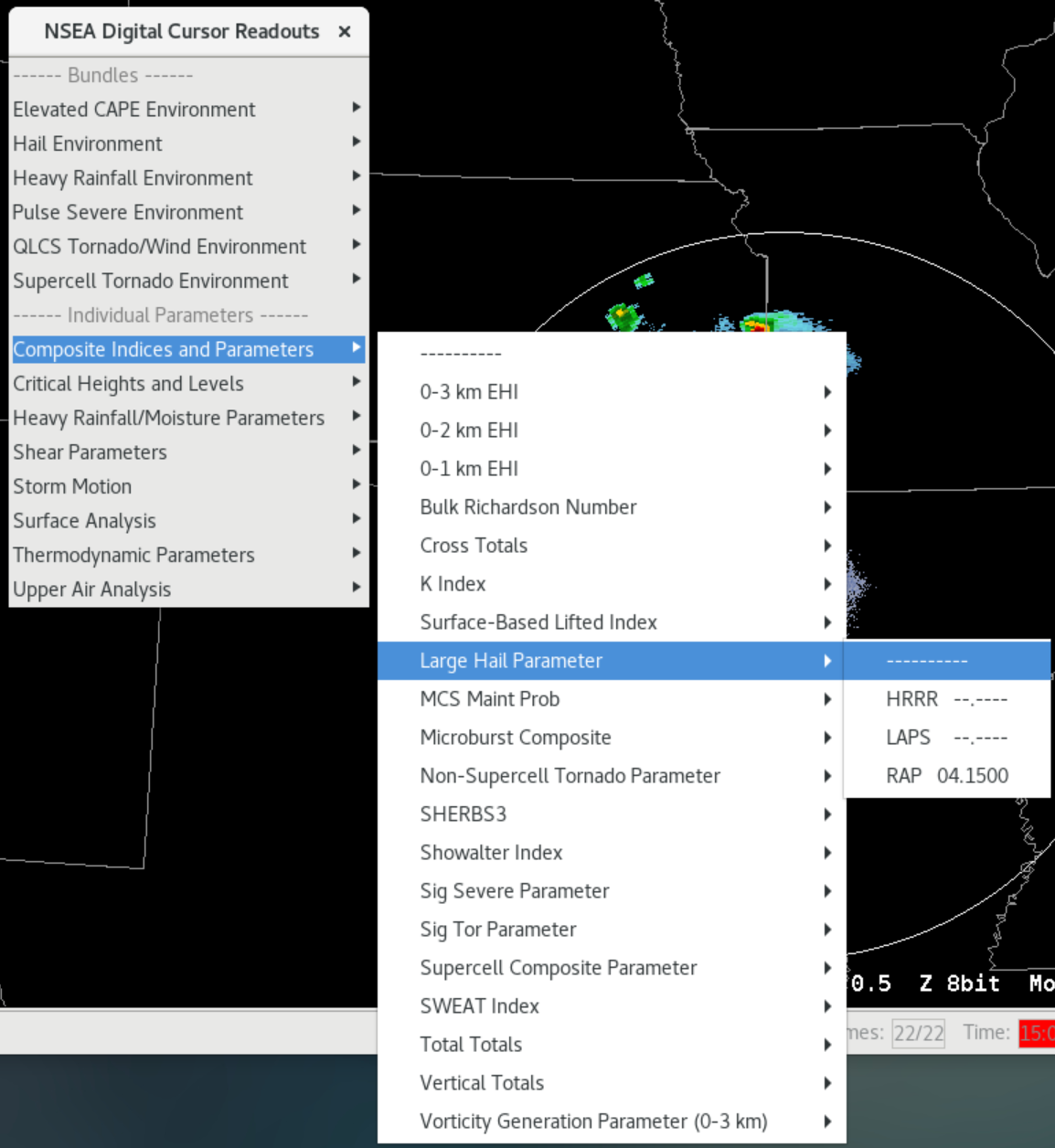
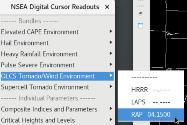
The default model choices for individual parameters are the High-Resolution-Rapid-Refresh (HRRR), Local Analysis and Prediction System (LAPS), and Rapid Refresh (RAP).
You want to choose the option that is going to give you the best estimate of the environment. LAPS is the local objective analysis software that runs in AWIPS which uses the RAP 1hr forecast and all your local data to objectively analyze your environment. LAPS has the potential to provide the best objective analysis of the environment, but it can require managing some of the data quality feeding into it, so your mileage may vary. The RAP has been a consistent model to use for severe weather applications for this purpose, and the HRRR is a third valid option to use, particularly when you are interested in analyzing forecast values. If you don't know which of these provides the best estimate of environment, then RAP is the safest place to start, and LAPS needs to be monitored for how it handles noisy surface observations while HRRR needs to be watched for model feedback.
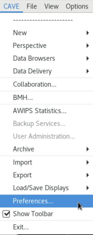
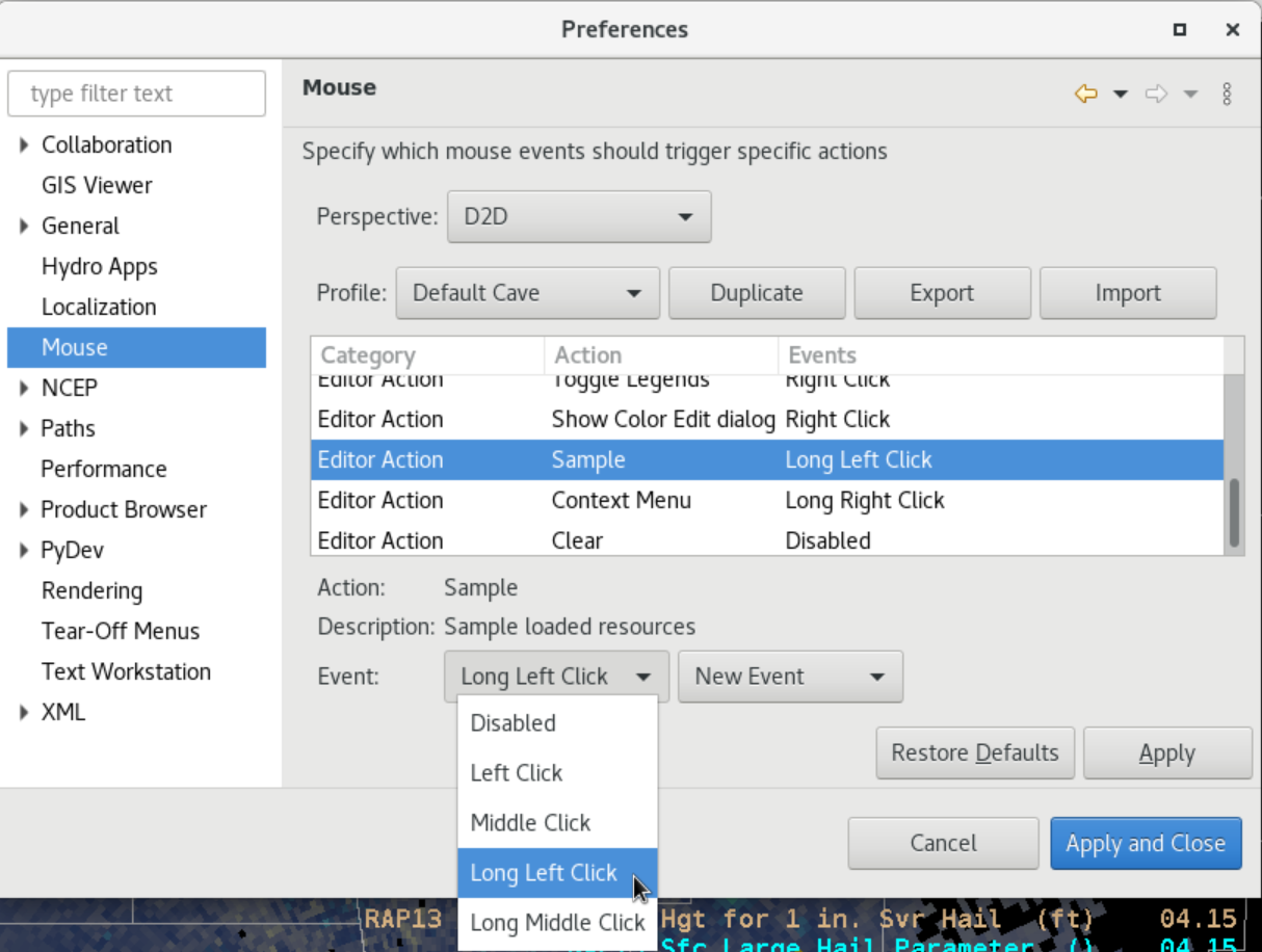
One tip for sampling on demand is to go to the CAVE->Preferences->Mouse setting (image) and select the Sample Action (image) and Long Left Click. Then click Apply and Close. Then you can long left click with the mouse button and roam to sample on demand rather than leaving sampling on all the time.
Loading Individual Parameters [Top]
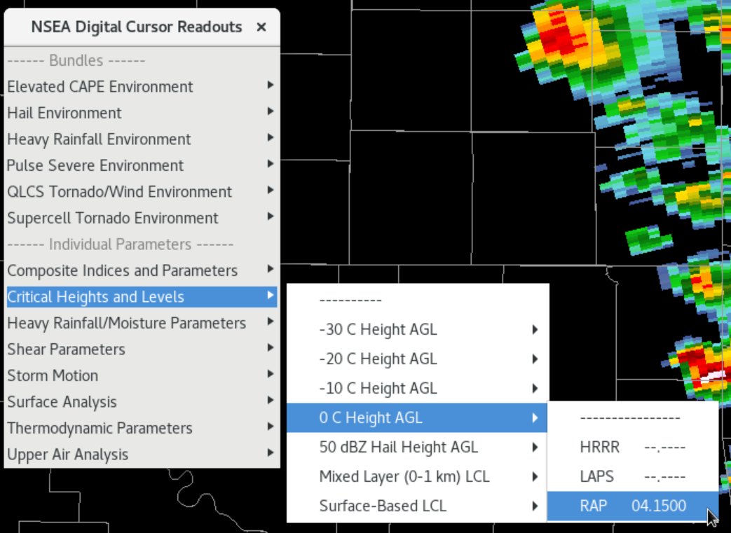
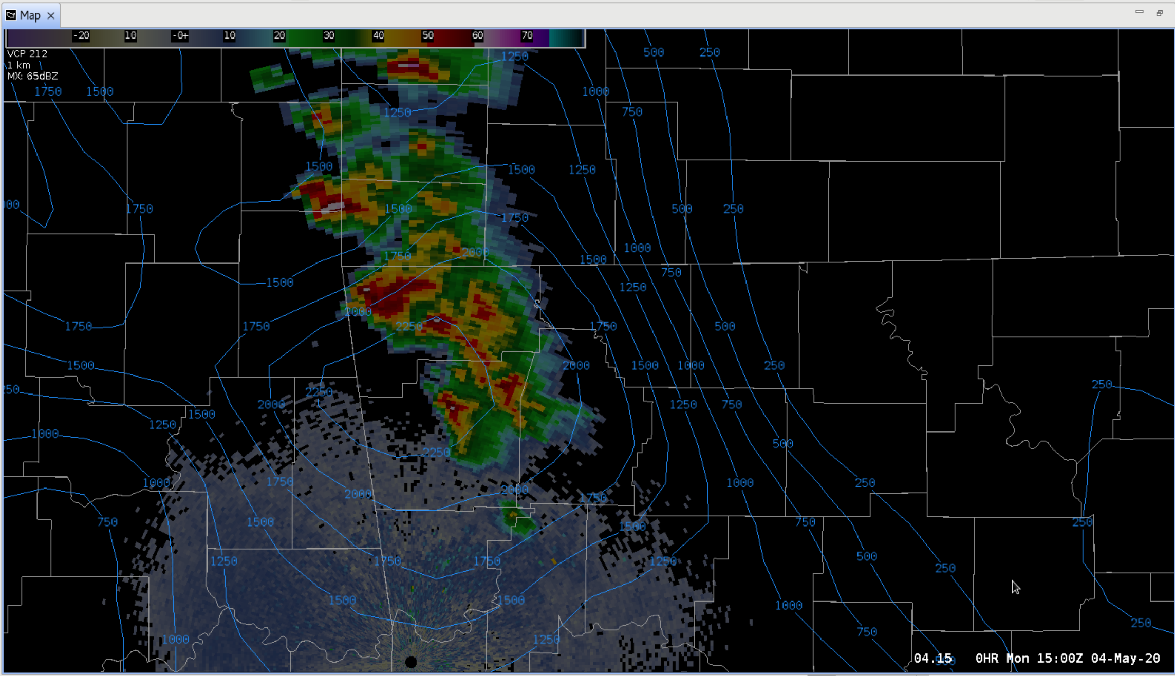
- Load any radar or satellite product of choice, and under the Volume->NSEA Digital Cursor Readouts->Critical Heights and Levels, choose the 0 C Height AGL and RAP. Then sample the image and notice that the data only displays when sampled.
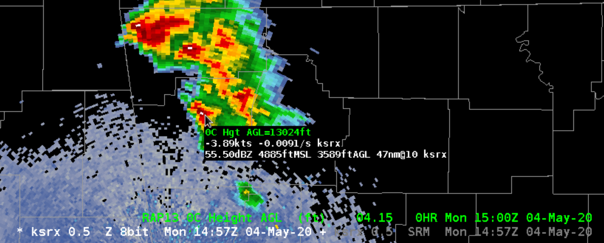
- The NSEA and Standard Environmental Packages both use a trick to hide the contours while allowing sampling by setting the default density for the product loaded to 0. Right click and hold on the text legend for the NSEA product and change the density from 0 to 1 to see the actual contours.
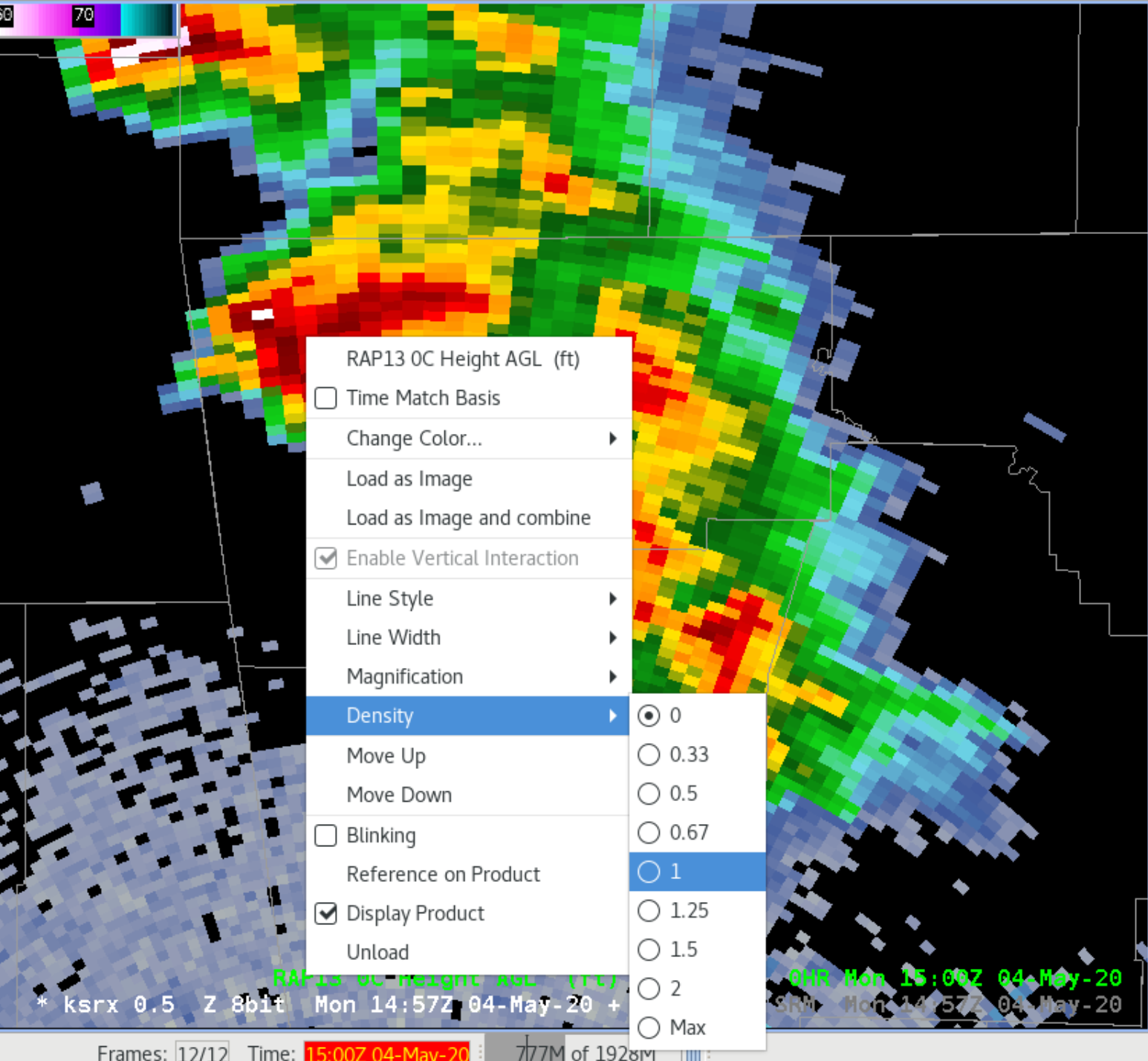

This can be a real handy way to load the contours for a single product. If you use the Density setting on the CAVE bar, that will impact all products loaded and can be messy when loading groups of parameters.
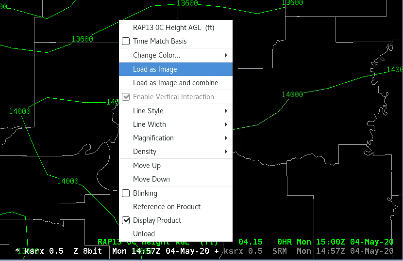
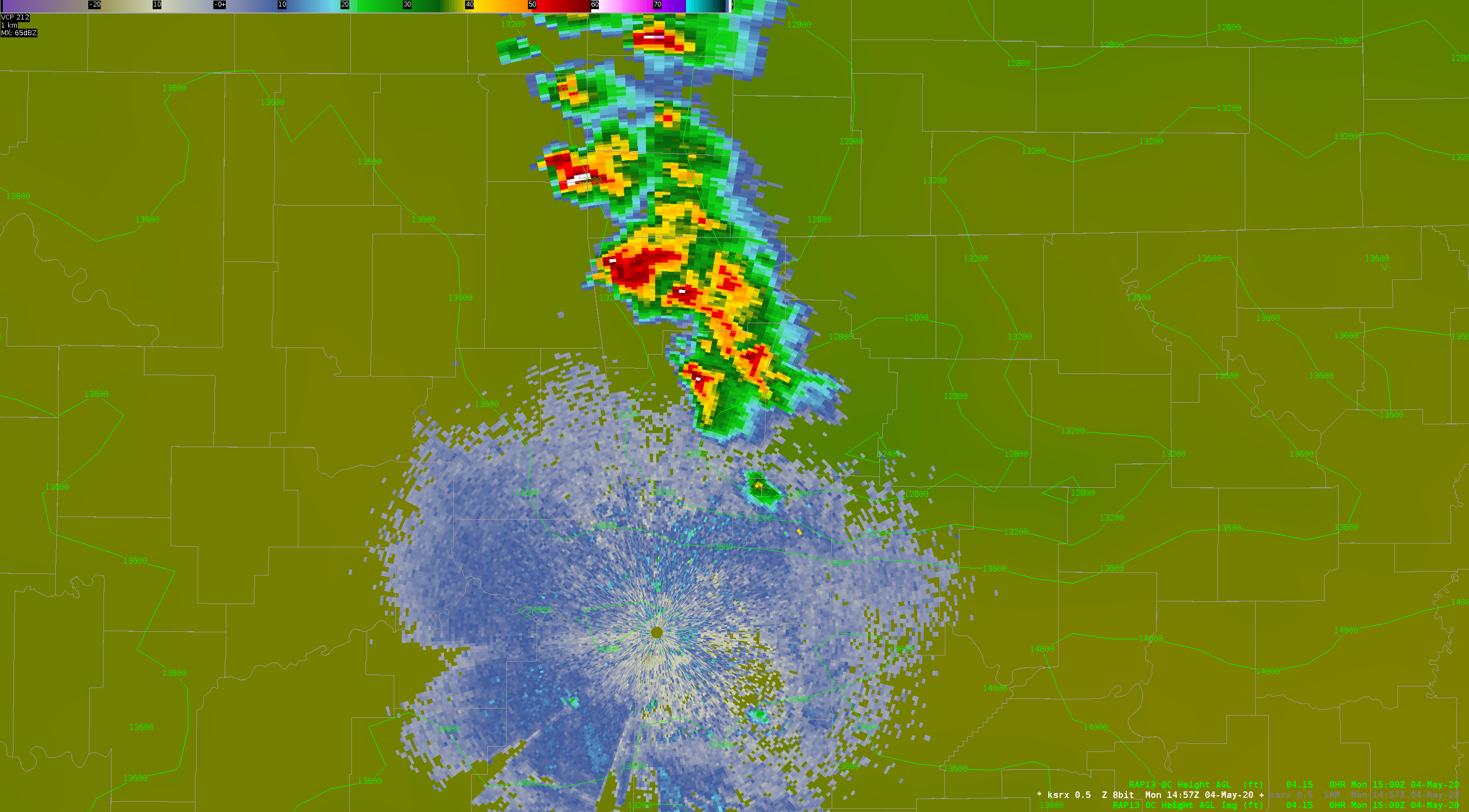
- Once you have a contour product, you can right click and hold on the text legend and select Load as Image to make an image out of it. Or select Load as Image and combine if you want to make a paired product if you have an image already loaded. You can also change Line Width, Line Style, Change Color, etc. to make contours more readable.
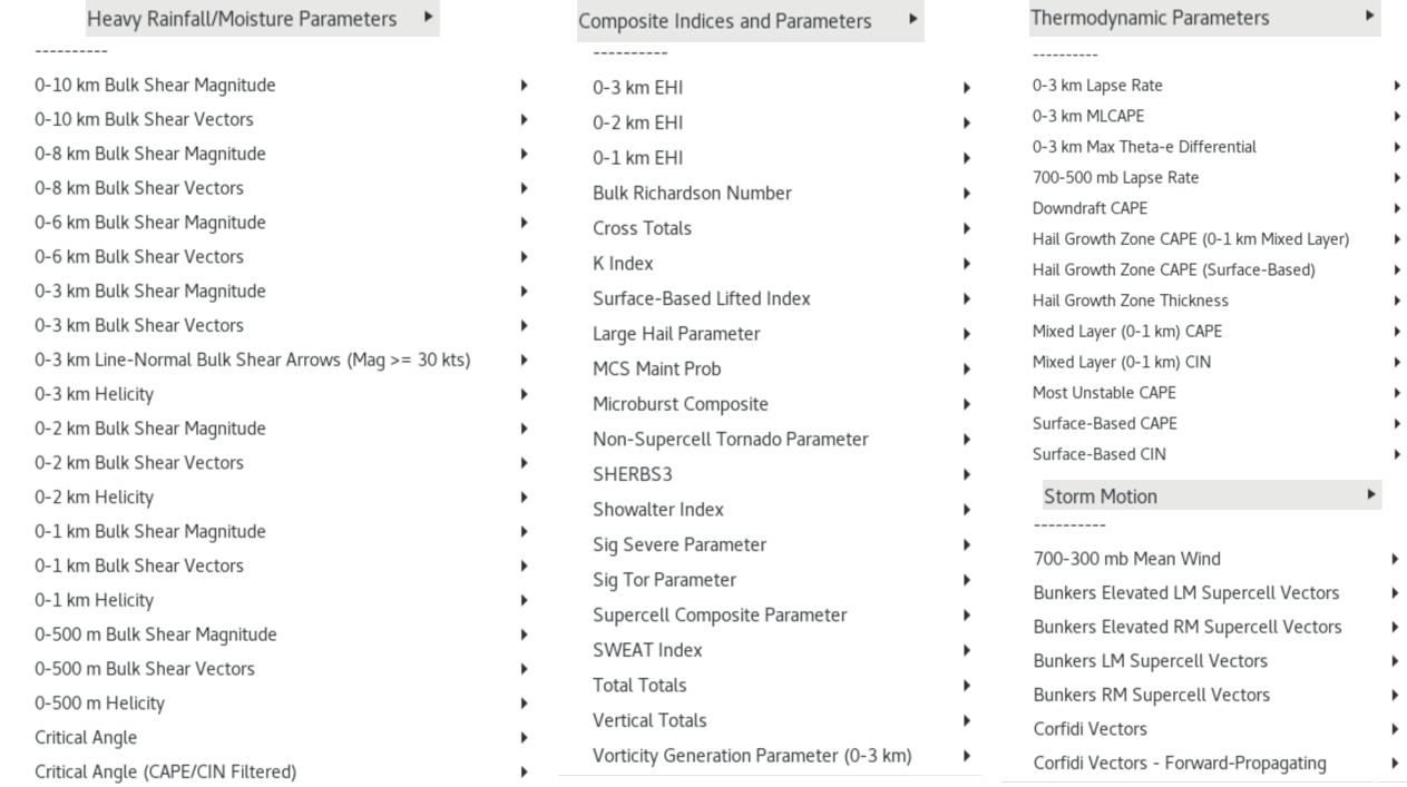
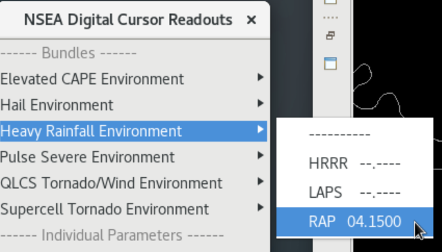
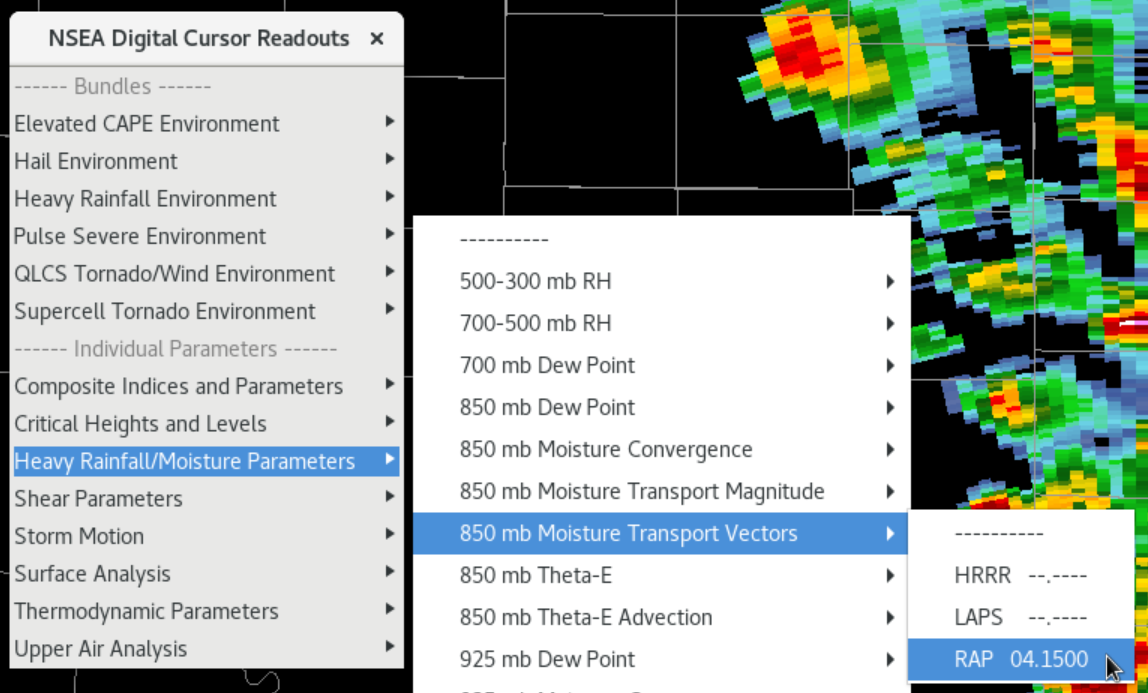
- Unload the new image you just created, and now under the Volume->NSEA Digital Cursor Readouts->Heavy Rainfall/Moisture Parameters menu, select 850mb Moisture Transport Vectors and RAP (image), and notice that vector arrows are plotted without sampling, and the magnitude is plotted in the sampling. These two examples illustrate the two different ways the NSEA is plotted.
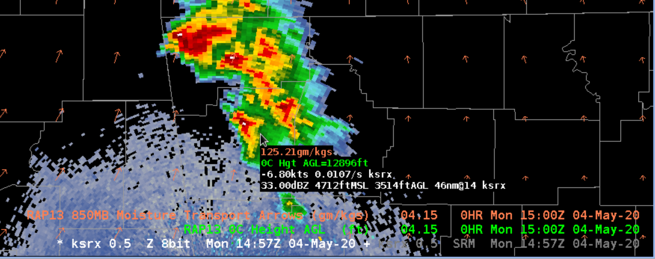
- Review each of the Individual Parameter groups to become familiar with individual parameters you can lightly overlay on any of your loaded data. Unload the Individual Parameters you try out when you are done.
Analyze Forecast Values [Top]
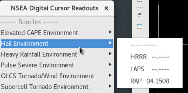
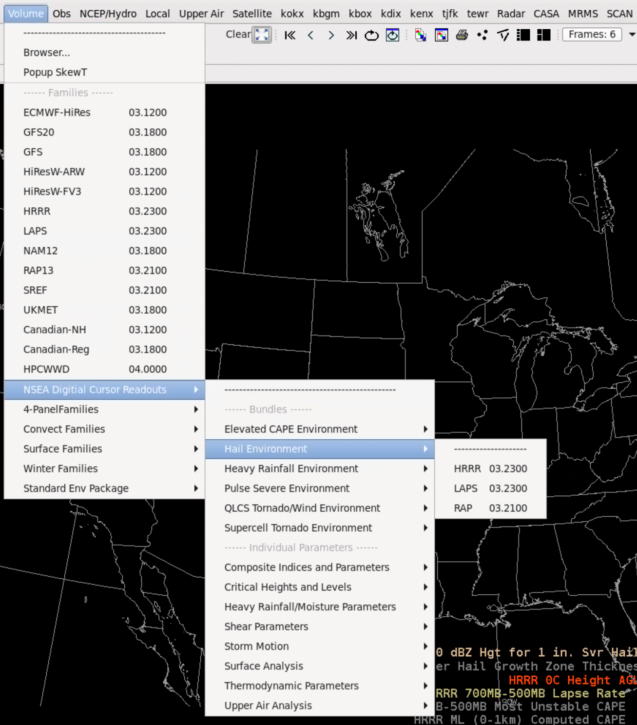
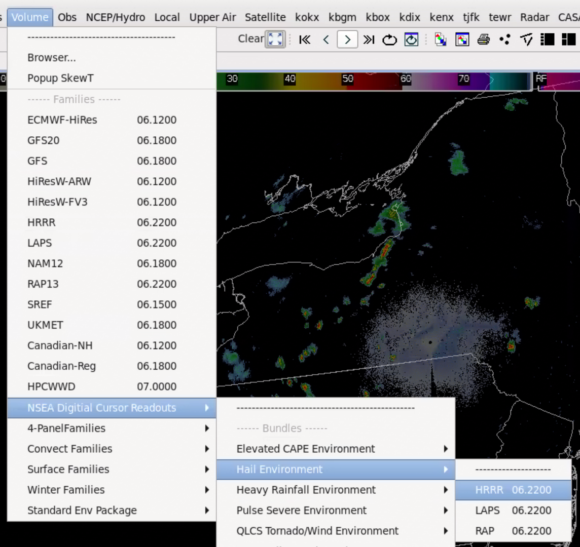
- If the Time Match Basis in the product legend is set to be the NSEA parameter, you can view the forecast values to quickly look hours ahead. This happens by default when you load the NSEA parameter in an empty editor. Start with an empty editor (e.g. hit Clear button). From the Volume->NSEA Digital Cursor Readouts->Hail Environment menu (image), load the HRRR.
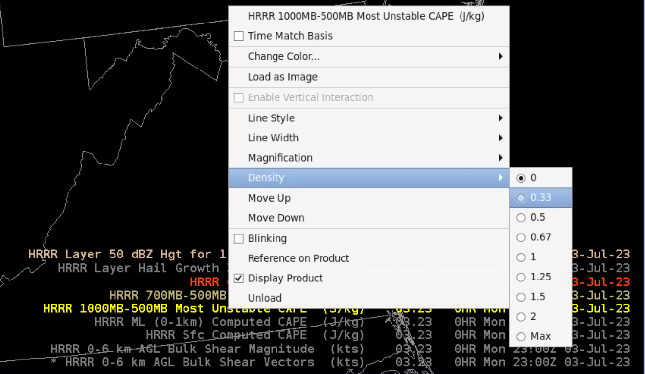
- Toggle on MUCAPE by clicking on the Most Unstable CAPE text legend. Then right click and hold on the Most Unstable CAPE text legend to change density from 0 to 0.33 (figure).
- Step through the loop and see how the MUCAPE forecast changes in the forecast.

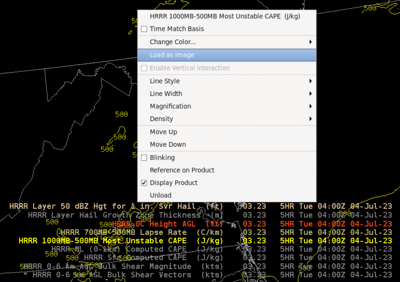
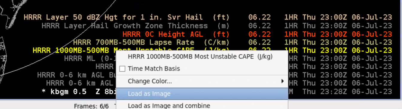
- Right click and hold on the MUCAPE text legend and select Load as Image (image). Sample the peak values. Clear the editor when you are done.
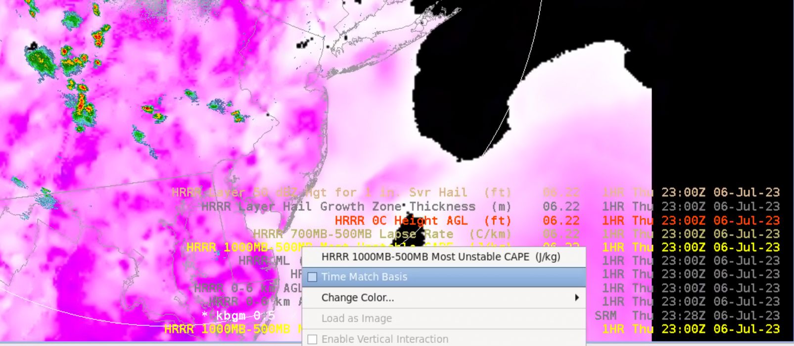
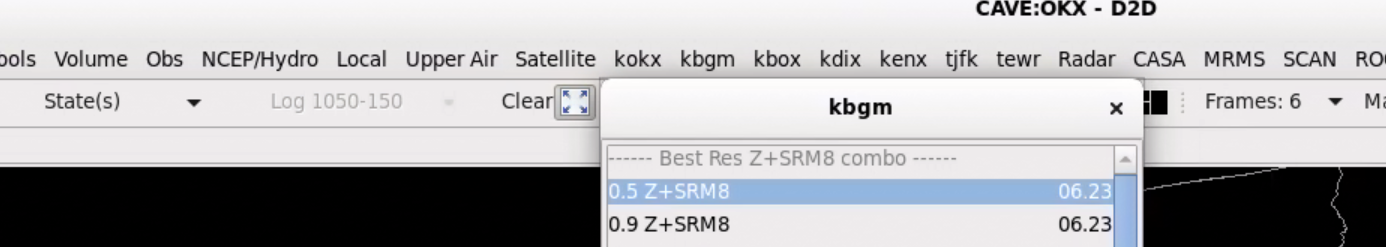
- Next we will show how to use the Time Match Basis to switch into forecast mode when NSEA model forecasts are paired with observations. Load a State scale 0.5 Z/SRM8 product from one of your radars and set the frame count to 6 (image) to support looking 5hrs ahead in a HRRR forecast.
- Load the Volume->NSEA Digital Cursor Readout->Hail Environment->HRRR (image), toggle on Most Unstable CAPE, and sample the radar image.
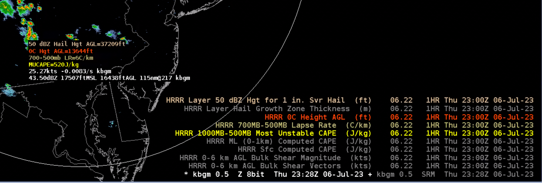
- Right click and hold on Most Unstable CAPE and select Load as Image (image) to better view the potentially noisy contours.
- Right click and hold on the Most Unstable CAPE and set that to be the Time Match Basis.
- Step forward through the forecast loop and see how the Most Unstable CAPE is forecast to change over the next 5 hrs. Sample the peak values.

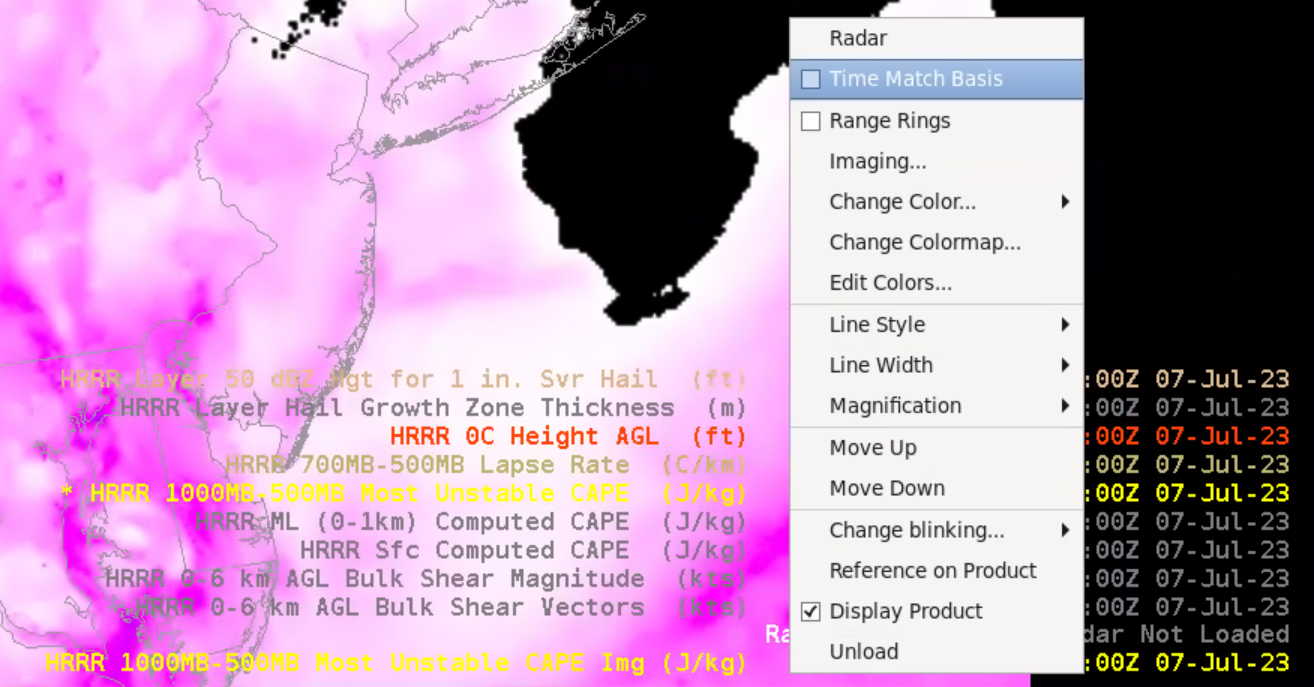
- To return back to the original radar sampling, right click and hold on the radar product legend and select it to be the Time Match Basis (image).
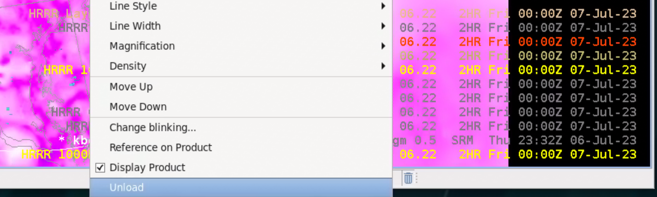
- Right click and hold on the bottom legend Most Unstable CAPE Img, and select Unload (image).
- Toggle off the Most Unstable CAPE legend, and sample the image as when it was first loaded.
- Realize the when you pair model forecasts with observational data, you can switch to the forecast mode by setting the model forecast to be the time match basis. Then reveal the contours by changing the density from 0 to non-zero and consider loading as image to make it easier to view.
Load Bundles [Top]
- The Bundles organization at the top of the menu are groupings of individual parameters by different environments. If you need some context around some of the parameters in their application for severe weather decision making, you can review the tornado, hail, and wind infographics in WDTD's Warning Methodology Handout and the flash flood infographics in WDTD's Flash Flood Warning Methodology document.
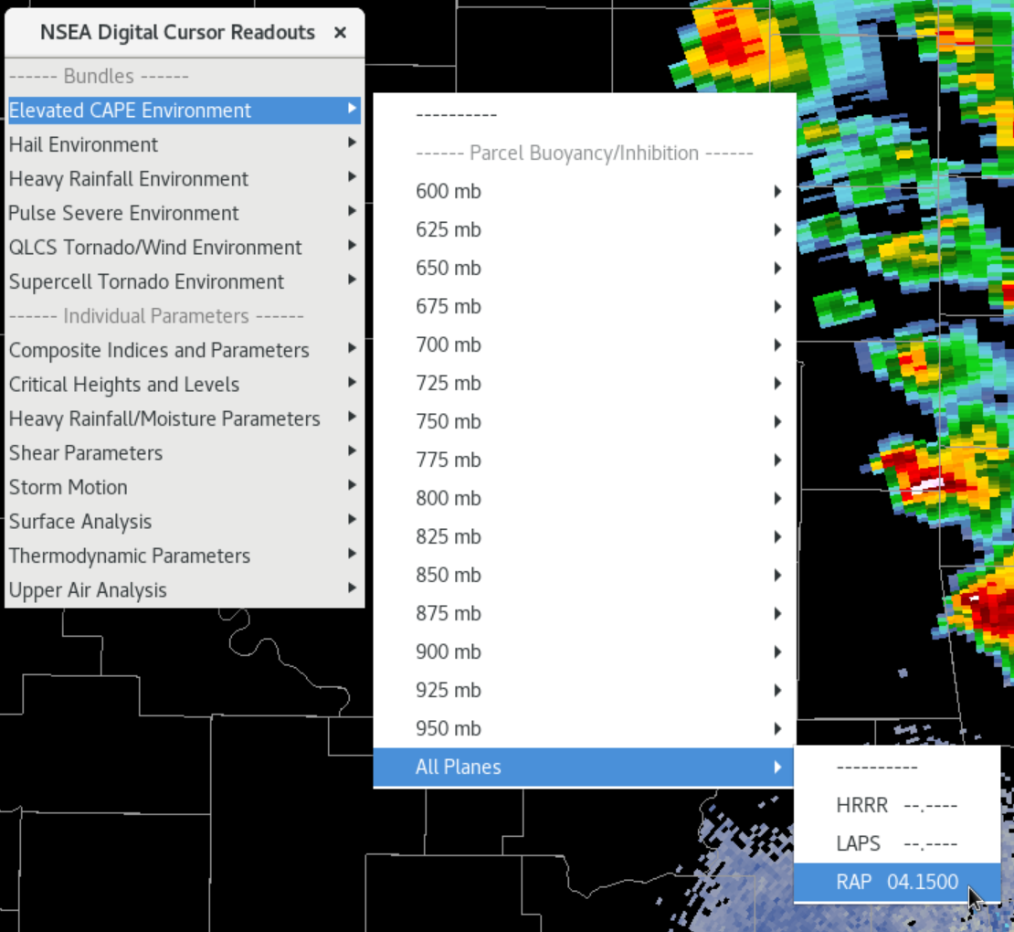
- The first NSEA bundle, Elevated CAPE Environment (Volume->NSEA Digital Cursor Readouts->Elevated CAPE Environment), at the top is a little different from the rest. It has lifted parcels from 950mb to 600mb and an All Planes menu. The All Planes can be a real handy way to identify peak elevated instability areas. Load a radar reflectivity product. Then click on All Planes and RAP to see this unique dataset.
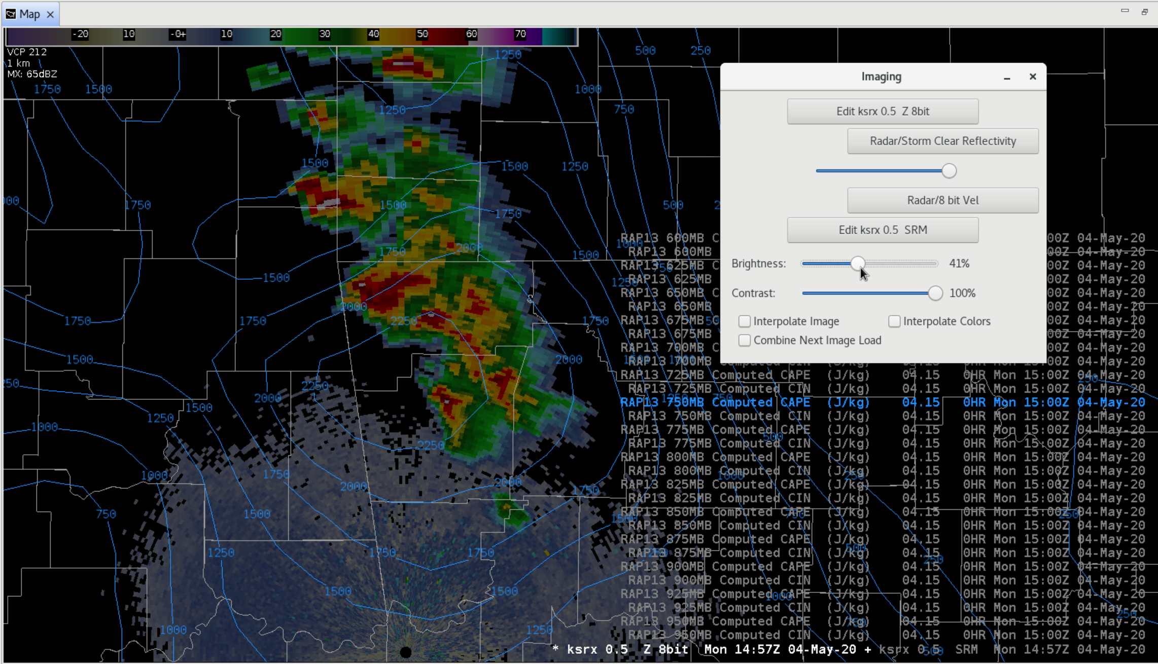
- On the keypad, click on 2-9 to toggle off the first 8 legends. Then hold down the Ctrl button and click on 0-9 to toggle off the next 9 legends. Then manually toggle off the rest of the legends. Start from the top and click on the Computed CAPE entries at different levels, and you can identify key layers of maximum buoyancy. In this elevated severe example, the surface CAPE was very low, and the maximum CAPE of 2250 J/kg was at 750mb. To be able to see the contours it can help to do a ctrl+i and dial down the brightness of the radar reflectivity in the imaging properties.

- Legend management is an important part of managing clutter with NSEA, though many of the bundles are not as extensive as this. You can always click on the Enter key in the keypad multiple times to cycle to just the time stamp. For this bundle it might be easiest to just use the clear button and reload the product and only load the new level you identified, but you can always right click and hold on each text legend and select unload to remove unwanted entries.
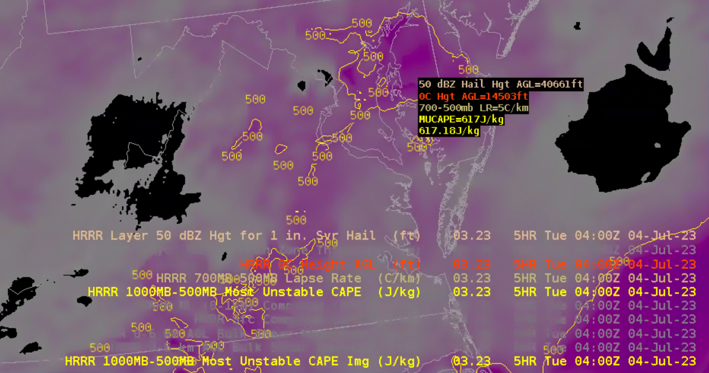
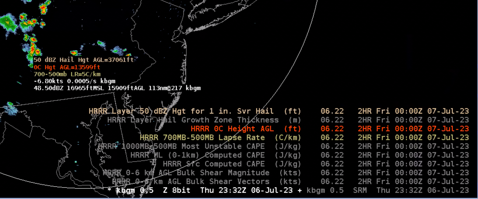
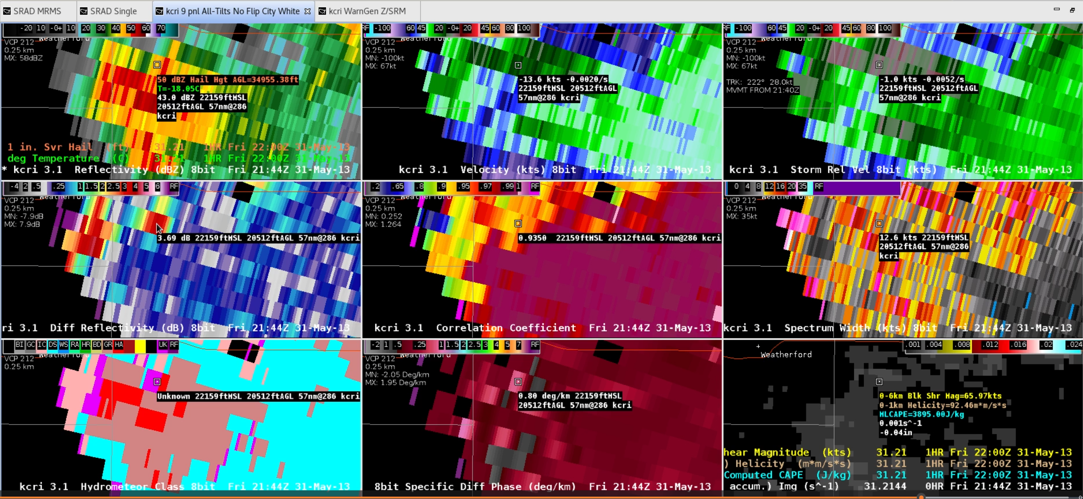
- Unload the NSEA overlay from the previous step (or use clear button and reload the radar reflectivity product) and click on the Hail Environment (image). Sample to review the parameters available for hail analysis.

There are many particularly effective parameters in this example. The 50 dBZ Hail Hgt indicates a 50dBZ height of around 35 Kft AGL is a good proxy for issuing a severe thunderstorm for 1" hail. The LHP indicates a risk for giant hail (greater than 4" hail was reported with this relatively weaker-looking storm which was actually the largest hail of the event). The 700mb-500mb LR of 8C/km indicates very strong lapse rates. Lots of other potentially useful parameters are toggled off like most unstable CAPE and 0-6km bulk shear magnitude.
- Hit the clear button and reload your display. Then click on the Heavy Rainfall Environment bundle and sample the image to review useful rainfall parameters.
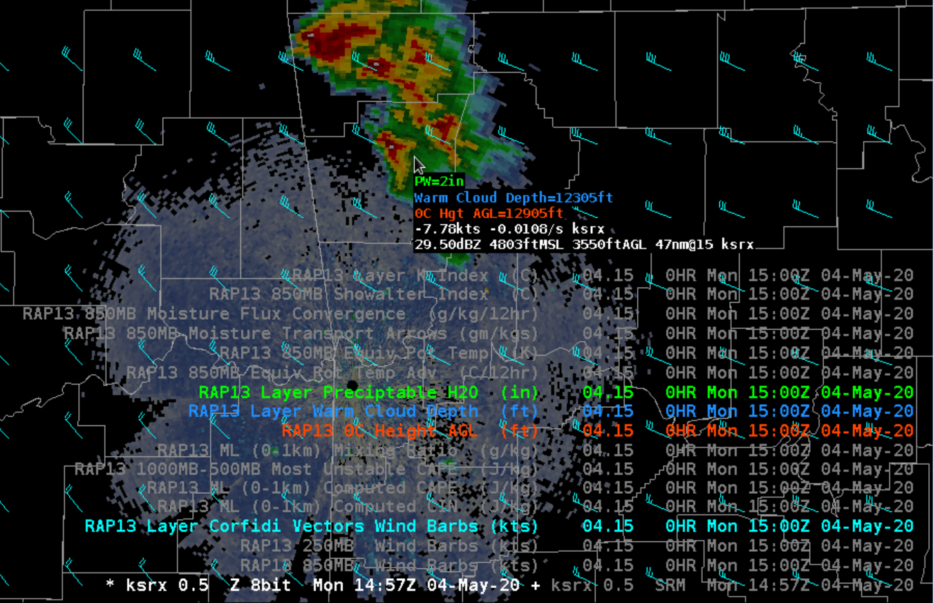
In this example, the 2" PW is relatively high for this time of year (above the daily max in climatology), and the warm cloud layer depth of 13 Kft is > 10 Kft which is supportive of very heavy rainfall. The mean wind calculations found under the NSEA Storm Motion section (not shown) indicate fast motions not supportive of heavy rainfall. This is also somewhat reflected in the moderate Corfidi vectors displayed by default in the Heavy Rainfall bundle, indicating any MCSs would not be particularly slow. Note many of the other available parameters that are toggled off by default. One important thing to point out is the default precision of the PWs is 1", and it rounds 0-0.49" to 0" and 0.5-1.49" to 1". So you really can't resolve the PWs very well outside of the 1" increments. This impacts some of the parameters in the NSEA.
- Hit the clear button and reload your display. Then click on the Pulse Severe Environment bundle and sample to review useful pulse severe parameters.

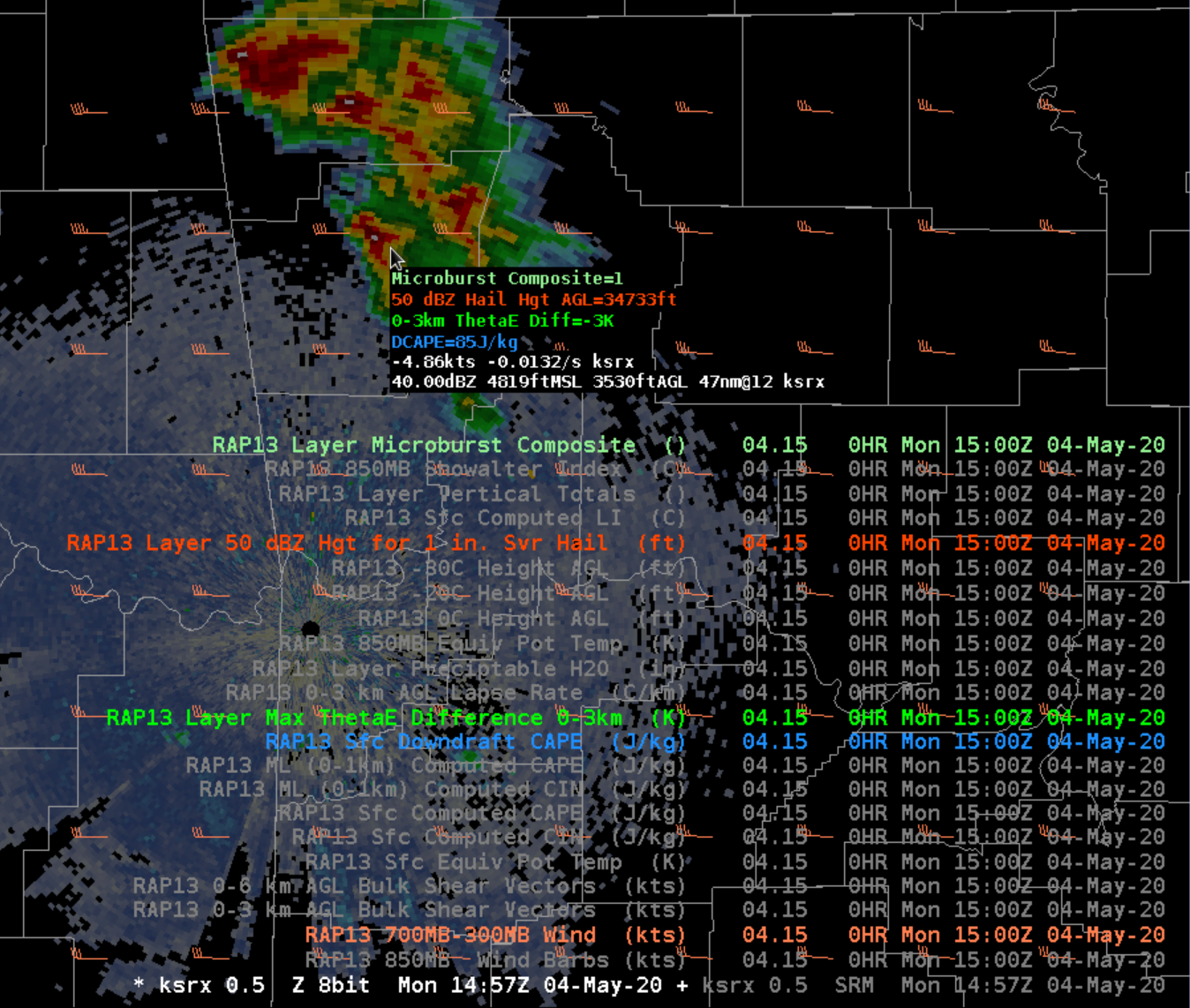
In this example the microburst composite of 1 is much less than 5-9; the 0-3km theta-E difference of 3K is << 25; and the DCAPE of 85 J/kg is << 900 J/kg for wet microbursts. This was a very humid elevated severe hail environment that did not produce any severe wind, and the parameters strongly suggested that should be expected.
- Hit the clear button and reload your display. Then click on the QLCS Tornado/Wind Environment bundle and sample useful QLCS parameters.
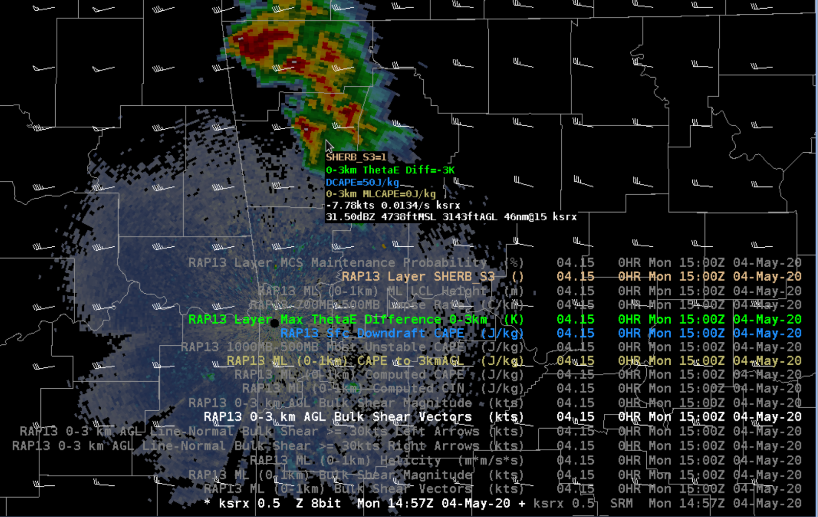
In this example the weak 0-3km theta-E difference, DCAPE, and 0-3km MLCAPE in the saturated and stable low-level air north of a surface boundary limited the damaging wind and mesovortex development potential in this case. The SHERB>1 and the magnitude of the 0-3km shear could be supportive of enhanced wind and mesovortex development if strong cold pools and a QLCS developed that were oriented perpendicular to the shear (more north-south oriented), but they didn't. The convection was mostly isolated supercells and multicells with no organized low-level wind structure or updraft convergence zones.
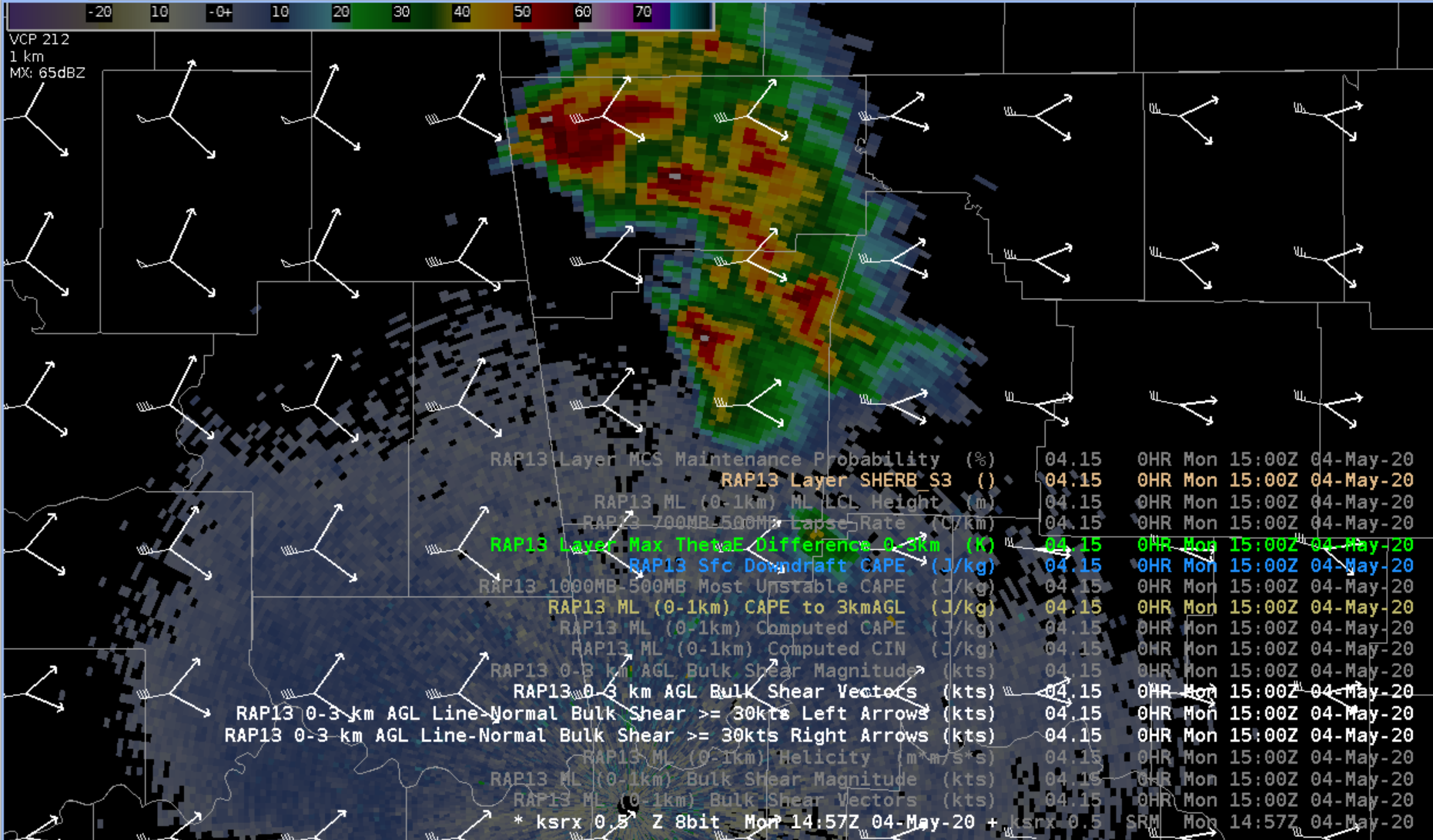
- The two Line-Normal Bulk Left/Right Arrows text legends that are toggled off by default are particularly useful for assessing the range of line-normal orientations supportive of 30kts of 0-3km shear and enhanced wind and tornado threat. Normally we would start by assessing the updraft convergence zone along the QLCS and then see if that vector perpendicular to that falls within the range of these two vectors, but there is no QLCS in this case. Toggle on the Line-Normal Bulk Shear vectors to see what this would be if we had a QLCS. Boundary normal orientations that fall within the range of these vectors are supportive. Instead of requiring a purely perpendicular (more north-south) line relative to the 0-3km shear vector, the two vectors below shows that a southwest-northeast oriented line would be supportive of the right arrow, and a southeast to northwest oriented line would be supportive for the left arrow.
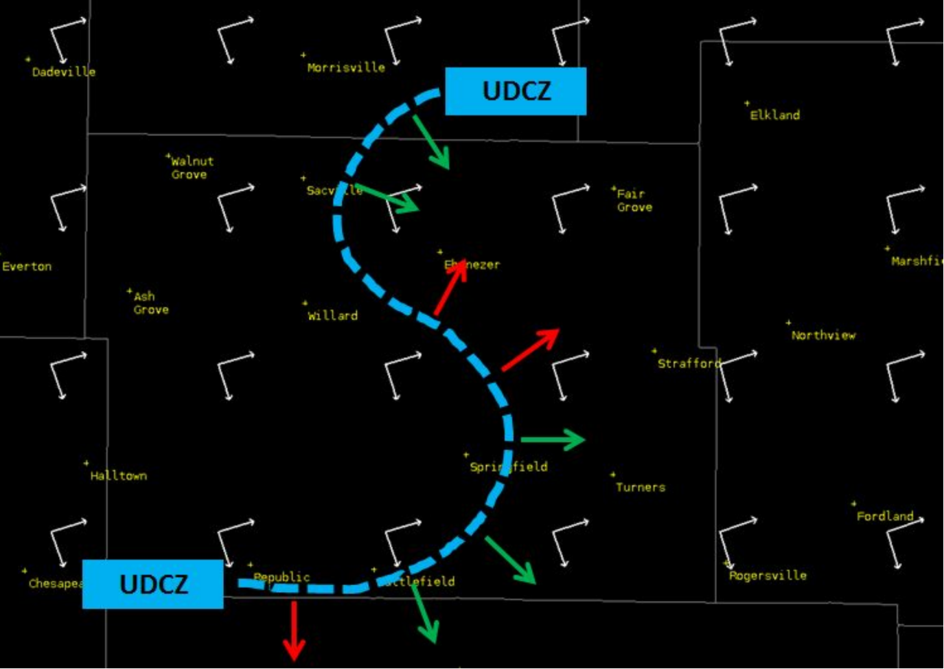
- Here is a diagram taken from the Tornado Warning Improvement Project training that illustrates favorable (green) and unfavorable orientations of the Updraft/Downdraft Convergence Zone (UDCZ) for a different example:
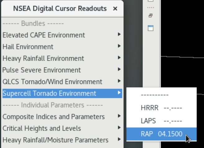
- Hit the clear button and reload your base display of radar/satellite data. Then click on the Supercell Tornado Environment bundle and sample to review useful tornado parameters.
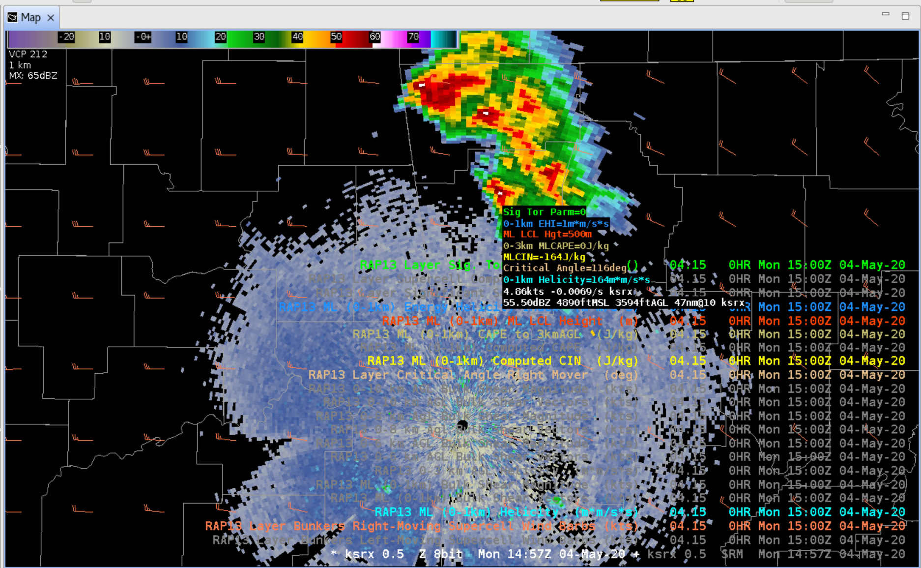
You will notice that the Bunker's right motions do not sample like the 850mb transport vectors. In this case the significant tornado threat was limited by the Sig Tor Parameter STP of 0, the large MLCIN of -164 J/kg, and 0J/kg of 0-3km MLCAPE. The ML LCL and 0-1km Helicity were supportive of tornadoes, but the lack of organized low-level rotation suggests those stable air parcels were probably not the ones feeding the elevated convection.
In these kinds of environments of strong CIN, effective-layer calculations are more appropriate. However, the AWIPS Volume Browser derived parameters that the NSEA uses does not calculate that. To find effective-layer SRH, STP, and bulk shear forecasters must use NSHARP in AWIPS or the SPC mesoanalysis on the Internet. The NSHARP sounding for the point being sampled above shows the fixed-layer STP was actually 0.8, and the effective-layer STP was 0 (see sounding below). It is important to point out the sampling precision is a full integer (0 or 1), and 0-0.49 is sampled as 0 and 0.5-1.49 is sampled as 1 which isn't ideal. 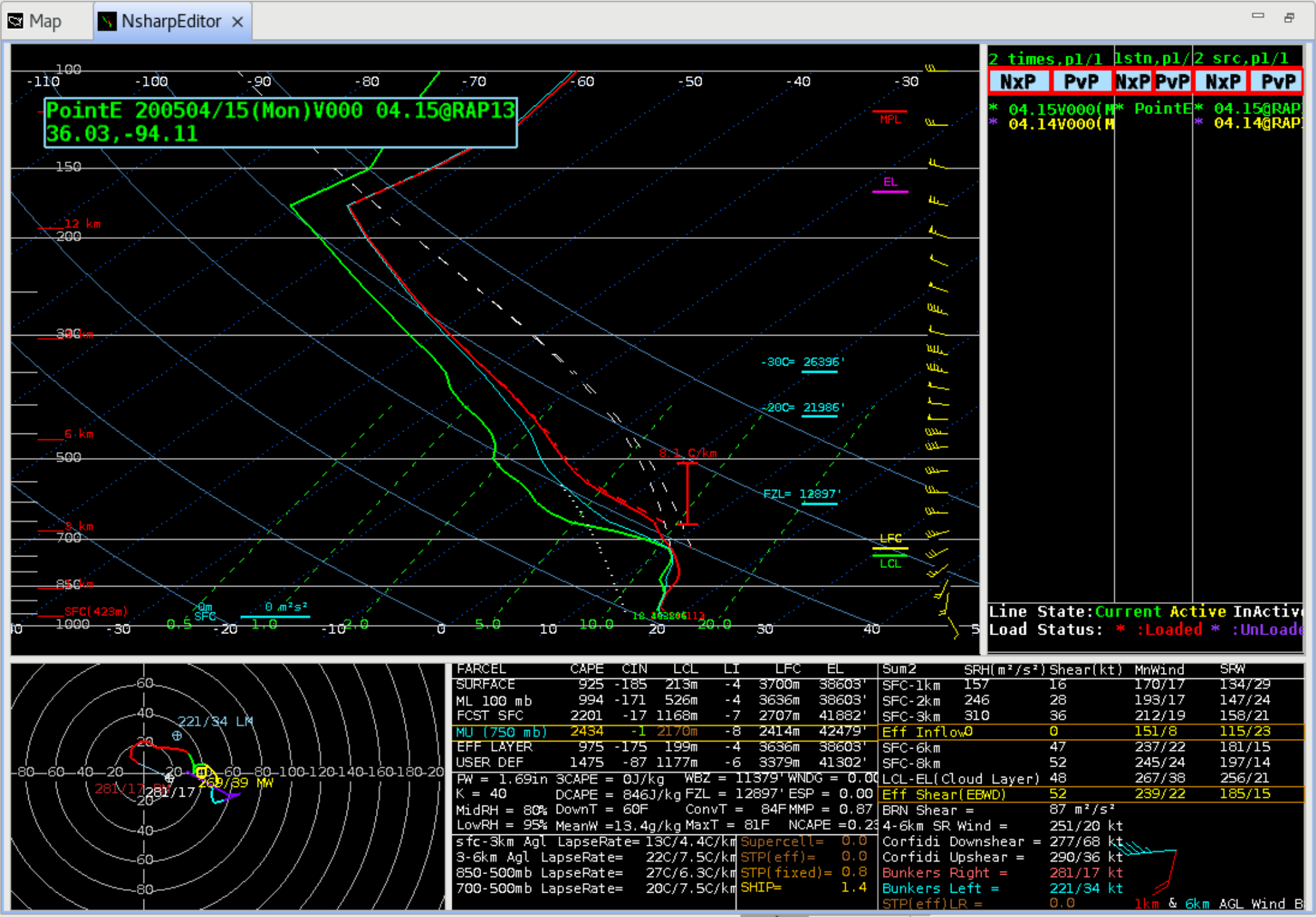
NSEA Digital Cursor Readouts Summary [Top]
- Summary: The NSEA Digital Cursor Readouts provides greatly simplified access to severe weather and flash flood parameters that can be loaded over any data and saved into procedures. The parameters can be time matched on top of existing data like radar/satellite, or the parameters can be set to be the Time Match Basis to enable analyzing parameter trends in model forecasts once contours are revealed by changing the density of a parameter to be non-zero.
The sampling provides a small but effective sampling footprint for most parameters though the integer precision values for parameters like PWs and STP are limited and will round 0-0.49 to 0 and 0.5-1.49 to 1. Some of the text legend grouping of the bundles can be large and obscure data or can be hard to read when toggled off. A good strategy to mitigate these effects are to toggle the legends off with the Enter key on the keypad when not needing to toggle the parameters, as well as reducing the brightness of the data that the parameters are loaded over. Right click and holding on the legend text and changing the density from 0 to something higher will turn the contours on if you want to see the spatial gradients. Once you have contour products loaded you can right click and hold on the text legend to change the line properties or Load as Image to convert the contour to an image, which can sometimes make a nice background field to plot a radar or satellite image layer on top of.
While some elements of elevated severe are uniquely supported like the elevated CAPE layers, the lack of effective-layer lifting methods in the AWIPS Volume Browser limits these types of severe weather analysis displays in environments with strong CIN. Thus, it is important to supplement Volume Browser-based analysis with NSHARP soundings and SPC mesoanalysis graphics.
Standard Environmental Packages [Top]
- The Standard Environmental Packages (SEP) work on a similar basis as the NSEA Digital Cursor Readout, but they load base state variables to the height of the radar data loaded. If you want to see the latest changes in SEPs due to a recent AWIPS bug, the example below will walk through adding temperature data to all tilts Z/SRM.
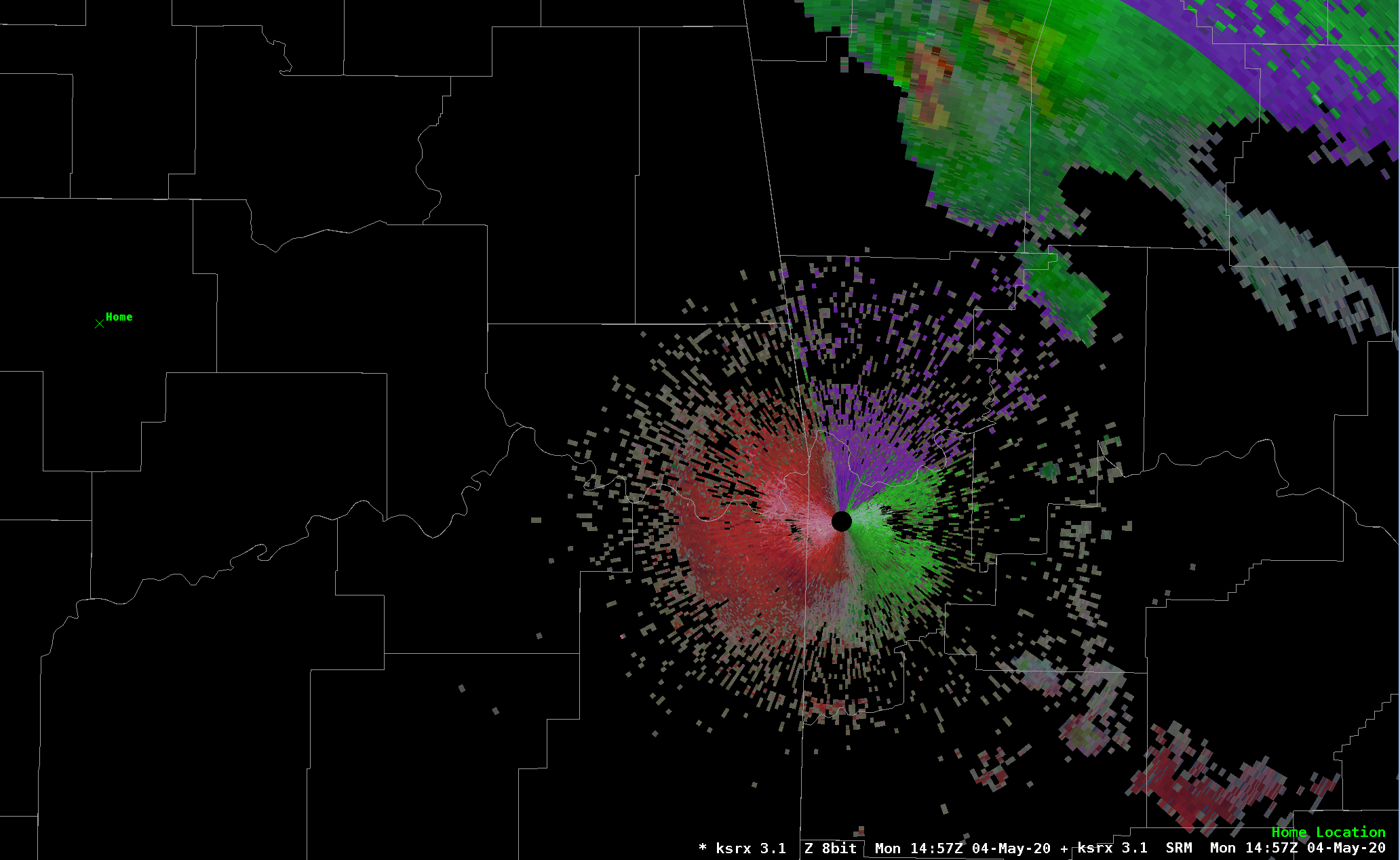
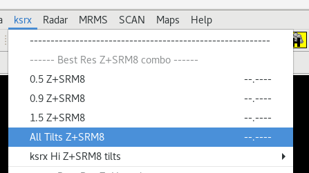
- From one of your radars, load All Tilts Z+SRM8 (image).
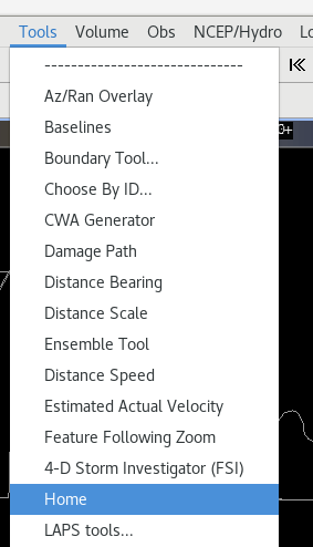
- When the Standard Environment Packages were first implemented, they were smart enough to use the radar loaded in the CAVE editor, but a new bug exists that requires you to move the Home tool to the location of the radar. From the Tools menu load Home (image).
- Make Home Location editable by middle clicking on the Home Location text legend or right click and holding on the text legend and selecting Editable.
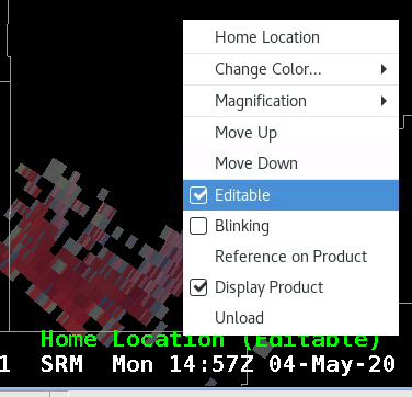
- Once the Home id editable, you can drag the Home location to the radar, or you can simply just right click on the radar location, and that will snap the Home id to the radar location.
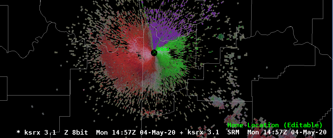
- From the Volume menu, load the Standard Environmental Package for the RAP13.

If you don't have the Home on the radar or it is close to a radar with no data on your AWIPS, you can sometimes fail to load any data. If your Home is close to another radar with radar data in the inventory, it may plot the polar data around the other radar location, which could be off your display if you are zoomed in.
- Toggle off Humidity by clicking on the Rel Humidity text legend, and then sample the data as you tilt through all tilts.
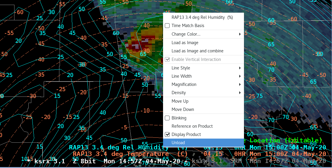
- Unload each of the Standard Environmental Packages for everything but Temperature by right click and holding on the appropriate text legend and selecting Unload (image).
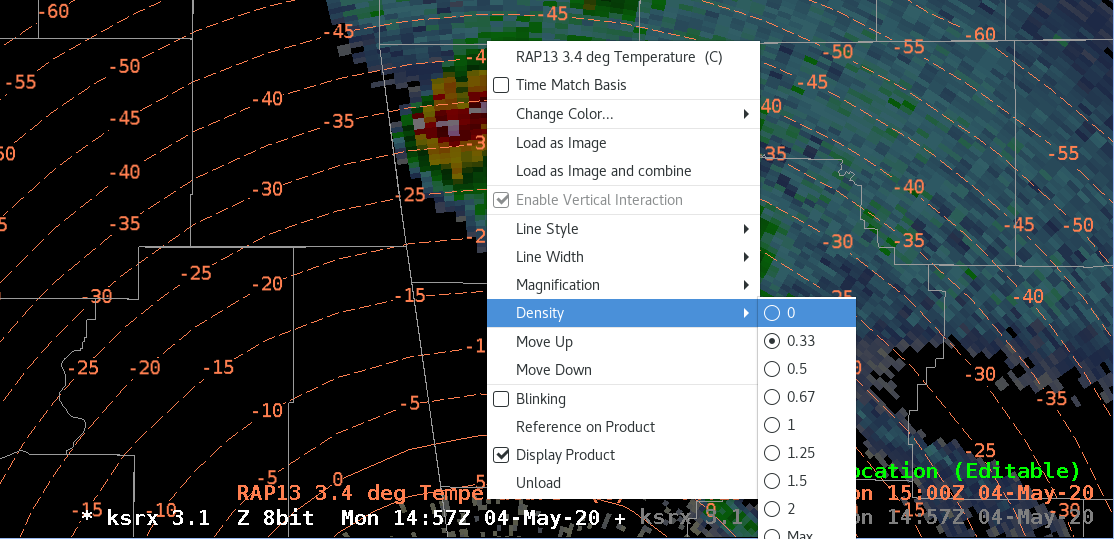
- Then right click and hold on the Temperature text legend and under the Density menu, change the Density to 0 (image).
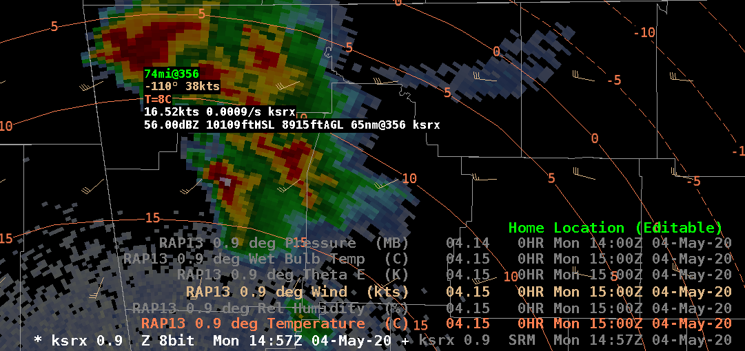
- Now sample the temperature data at the height of the radar data with the contours at 0 density. This is a handy way to provide sampling with no contours. You can always turn the contours back on by changing the density to something non-zero.
Procedures Examples [Top]
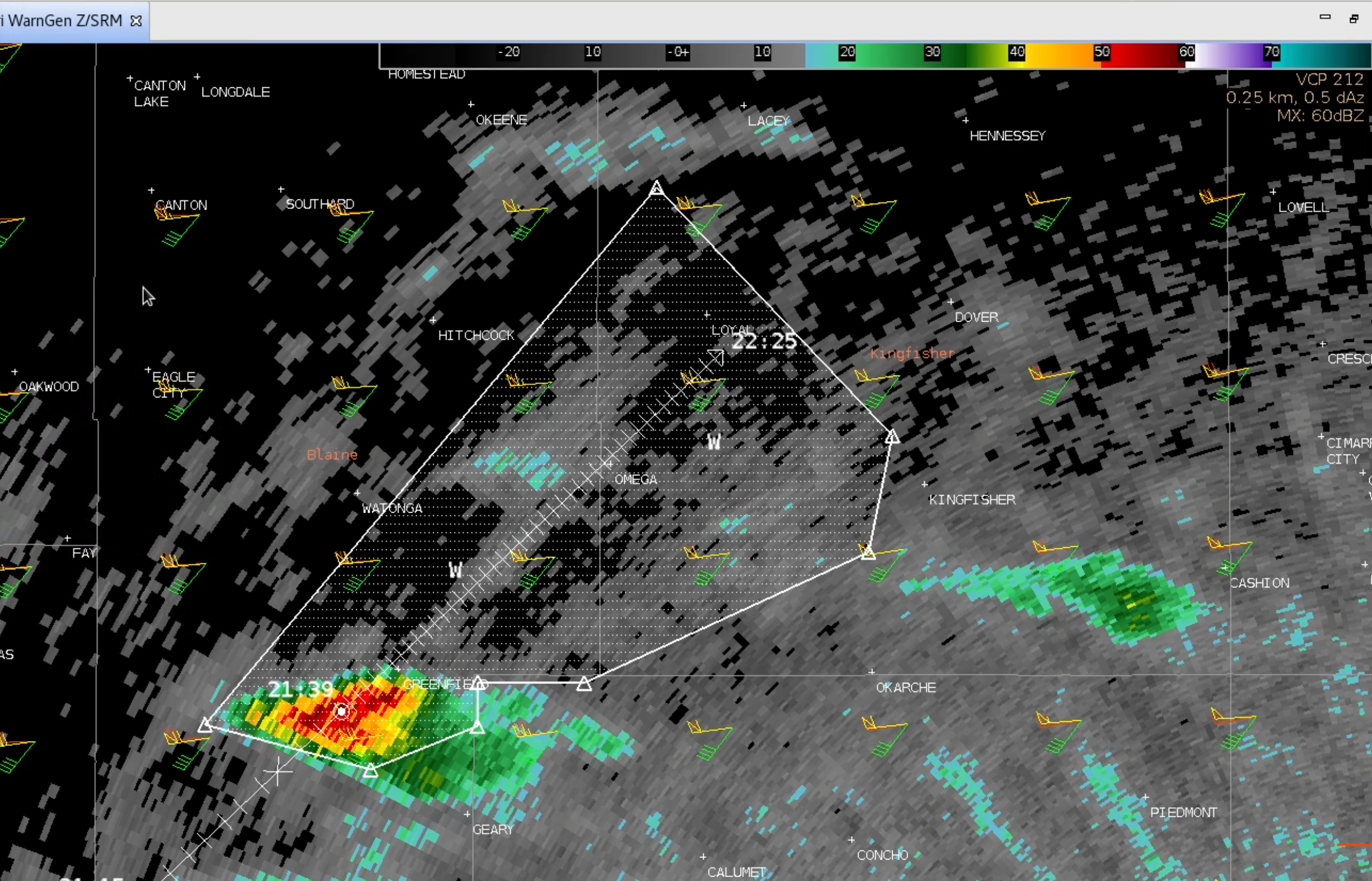
- There are many ways to integrate individual parameters into convective analysis bundles. WDTD has found two particularly effective approaches worth sharing. The first is to overlay the Bunkers left/right motions and 0-6km shear vectors over the WarnGen display. This provides a way to visualize the likely ranges of storm motion and adjust the right and left side of the polygons accordingly.
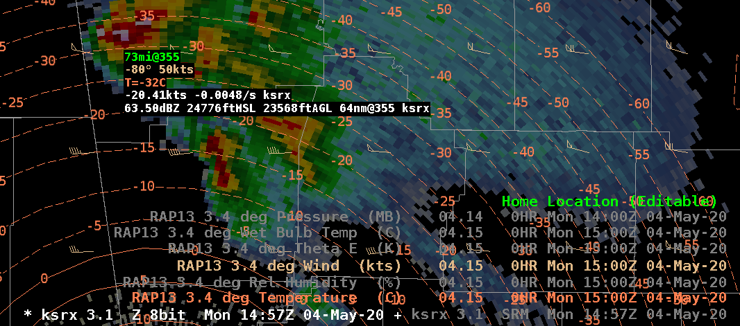
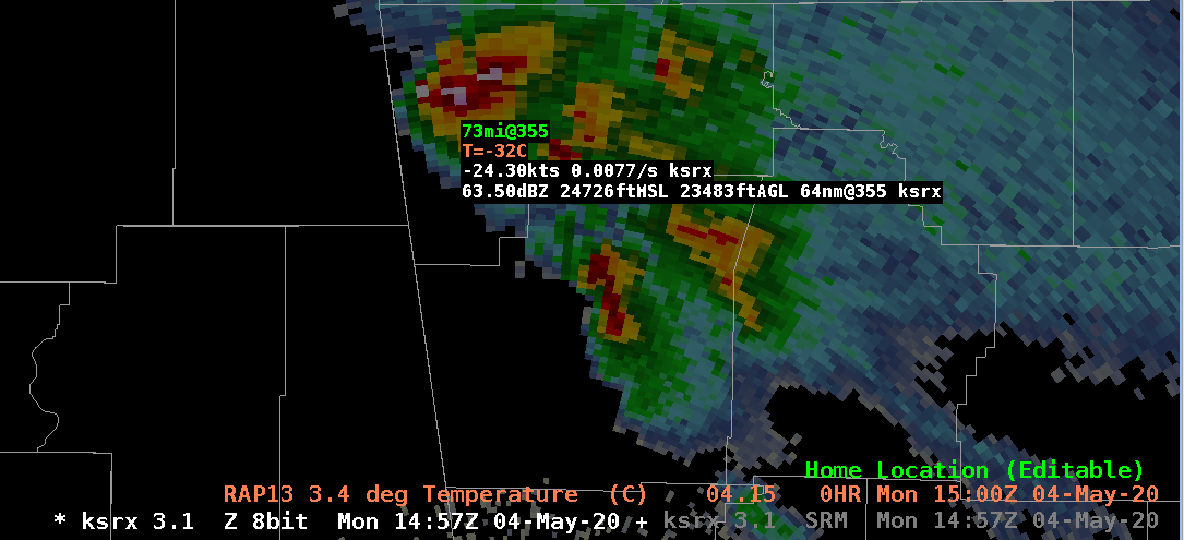
- Another technique is to overlay the height of the 50dBZ hail on the all-tilts reflectivity panel along with the temperature loaded from the standard environmental package. This allows quick assessment of severe 1" hail, and it provides a thermal reference for high reflectivity cores aloft.


