This lesson presents information on the Flash Flood Monitoring and Prediction (FFMP) application. This includes a synopsis of the High-resolution Precipitation Estimator (HPE) and the High-resolution Precipitation Nowcaster (HPN). While this lesson presents the basics, more detailed tasks and examples are included in WES Exercise #7(Flash Flood Monitoring and Prediction) on your local WES-2 Bridge machine. RAC will also provide substantial training on FFMP and its inputs, and this lesson is intended to cover the basic procedural knowledge to interrogate precipitation estimates with FFMP.

Required WES Exercise #7 (Flash Flood Monitoring and Prediction (FFMP))

About FFMP

The Flash Flood Monitoring and Prediction (FFMP) system allows you to interrogate radar precipitation estimates and compare to flash flood guidance (FFG) and average recurrence interval (ARI) data on a user-specified duration in support of flash flood warning operations. River Forecast Center FFG is the amount of precipitation required for a given duration to cause flash flooding (e.g. 2.5" in 1 hr). ARIs are the recurrence intervals in years for a given precipitation amount over a given duration (e.g. a 4.2" accumulation in 3hrs occurs every 10 years). FFMP conducts its precipitation analysis on a basin-scale, meaning that all of the calculations are done over the area of a drainage basin or larger areas of basin aggregations called Hydrologic Unit Cycle (HUC) layers. 

Starting FFMP Table

All of the FFMP product suite products are available underneath the SCAN menu in the D-2D perspective of CAVE. The FFMP products are grouped together in the “FFMP” section and they are grouped together by quantitative precipitation estimate (QPE) input source. FFMP is configured to use any of your WFOs dedicated radars’ DHR and DPR data as a QPE source, and it is configured for displaying the High-resolution Precipitation Estimator (HPE) and Bias High-resolution Precipitation Estimator (BHPE). The Multi-Radar Multi-Sensor (MRMS) is another QPE source that uses the Surface Precipitation Rate (SPR) products.

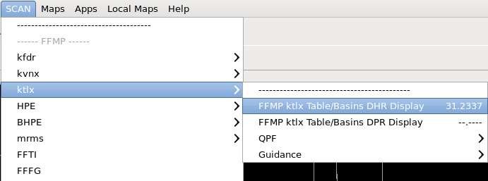
FFMP can display Quantitative Precipitation Forecast (QPF) data under the QPF menu which are all 1hr forecasts by default. While QPF data is difficult to use because of its accuracy (note: MRMS QPF doesn't exist and the menu should not be there), the best QPF source is the HPE Nowcast which uses a sophisticated precip tracking and extrapolation scheme. Under the Guidance menu, the RFC FFG for a given day can be loaded as well as the static ARI precipitation values for different intervals (e.g. ARIFFG100->FFMP ktlx ARIFFG100 3.0 HR Display will load the precipitation map for a 100-year precipitation recurrence interval over a 3hr duration). 

After selecting a FFMP Table/Basins Display product to load, FFMP displays a GUI, called the FFMP Basin Table, and an interactive image in the main display panel of the D-2D perspective.

The FFMP Basin Table

The FFMP Basin Table contains comprehensive data on all the drainage basins in your CWA at multiple spatial scales (uses FFMP Basins->FFMP Small Stream Basins and FFMP Small Stream Basins Links maps visible under the Maps menu).

need new image with all and only small basins configured and the letters i, ii, iii, iv annotated per text below (see previous year)

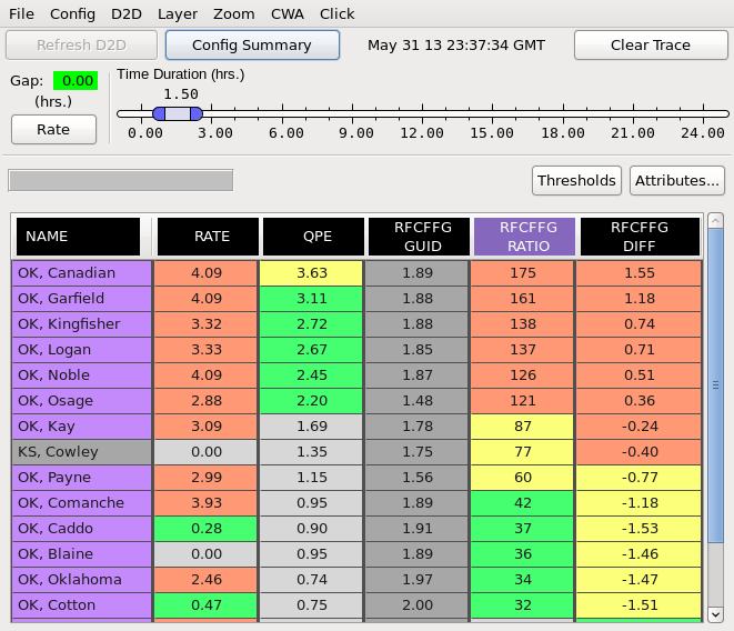
The GUI is divided into five different sections, each discussed below.

Menu bar

The Menu bar (referred to by label "i" in the FFMP GUI image) contains numerous menu buttons that allow users to access many functions and features in FFMP. Many of the menus are not routinely used, but some are used more than others:

• File - Used primarily to save or retrieve FFMP configuration settings.
• Config - Allows users to change the FFMP configuration settings for Link to Frame (i.e., time matching between FFMP Basin Table and main display), Worst Case (aggregate FFMP data will show worst case data vs. average), and Auto-Refresh.
• D2D (commonly used)- Changes what attribute is used to fill county and basin level plots in the main display (typically change between QPE, ratio, and diff to analyze flash flood threat for different durations).
• Layer (commonly used once)- Allows users to change how FFMP Basin Table and Color Image aggregate (i.e., average) data (typically use All & Only Small Basins for primary analysis and County aggregation when identifying individual basin names).
• Zoom - Changes settings for how FFMP Basin Table and Color Image behave when a user selects a county in the Basin Table.
• CWA - Allows users to trim the Basin Table and Color Image down to only counties and basins in a particular CWA.
• Click (commonly used)- Configures interactivity available to users when they click on the Color Image in the main D-2D display (display upstream and/or downstream basin trace or display basin trend graph).

Utility bar

The Utility bar (referred to by label "ii" in the FFMP GUI image) contains three buttons (“Refresh D2D,” “Config Summary,” and “Clear Trace”) and the date/time for the currently displayed data. These buttons are infrequently used. “Refresh D2D” will update the Color Image in the main display panel of the D-2D perspective if you turn off the Auto Refresh. Selecting the “Config Summary” button will display a pop-up window with the current settings for several of the FFMP configuration properties. “Clear Trace” clears the basin trace in the display if you generate one.

Time Duration

The Time Duration section of the FFMP Basin Table GUI (referred to by label "iii" in the FFMP GUI image) allows users to configure the duration of the precip accumulations and flash flood guidance (FFG) displayed in the table and in D2D (e.g. 1hr accumulations, 2.5hr accumulations). The “Gap” value indicates the cumulative amount of time (in hours) that data are not available for the specified duration window. The “Rate” button toggles on/off the display of instantaneous precipitation rate information (i.e., Time Duration = 0 hrs) in the Color Image display (Note: The Table Body in the FFMP Basin Table will be void of any data when the “Rate” feature is activated).

Attribute Column Titles and Buttons

The attribute column titles (referred to by label "iv" in the FFMP GUI image) are the labels designating which attributes are displayed in the Table Body. Selecting the Title of an attribute sorts the data in the Table Body by that column. You can select which attributes you want to display in the table body by selecting the “Attributes...” button, but most of the time this is not used. In the Attributes GUI, you can select which products you want to display in the FFMP Basin Table GUI.

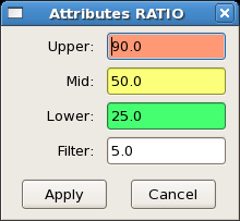
If a county’s or basin’s data for that attribute falls below a predefined “Filter” value, that county or basin will not be displayed in the Table Body (except when sorted by Name, then all counties/basins will display in the table). FFMP allows the user to configure the attributes displayed in the Table Body by using the Attribute Inclusion GUI. The “Filter” value, as well as other threshold values used to color code the data in the Basin Table, can be accessed and/or edited through the “Thresholds” button. When selecting the “Thresholds” button, five menu items will appear (RATE, QPE, QPF, RATIO, and DIFF). Press the Left-Mouse button over any of the attributes, and an Attributes GUI will appear. These defaults are typically pretty good, so this is not routinely changed.

The Table Body

FFMP lists the precipitation and guidance data (either FFG or ARI)flash flood guidance data for each drainage basin in the Table Body, and it can also be used to display ARIs. If there is no rainfall over all the geographic entities for the specified precipitation data source and time duration, the table indicates “NA”. The main display is linked to the table. After pressing the Left-Mouse Button on an identifier in the “Name” column of the Table Body, the main display panel zooms and re-centers on that particular county or basin and places an “X” at the centroid of that geographic region. The D2D display can be sampled, and it will match the contents of the table when they are linked (controlled by Config->Link to Frame option).

FFMP Basin Trend Graphs

One of the more complex analysis tools of FFMP is the basin trend graph. The basin trend graph allows you to view multiple attributes of a single basin within a graphical representation of rainfall with respect to time. The GUI is divided into three different sections, which will be discussed below.

Trend Graph

The trend graph (referred to by label "i" in the FFMP Basin Trend image) plots the time (hours; x-axis) vs. the rainfall accumulation and/or rate (inches and/or inches per hour; y-axis). The default basin trend graph plots the instantaneous rainfall rate (blue line) and the running QPE accumulation (black line with color fill) with respect to time. The time axis starts with Time = 0.0 hours on the left and scrolls over to Time = -24.0 hours on the right (with “All hr.” selected). However, reading the time axis has a few different meanings depending on which attribute you are analyzing:

• For Rainfall Rate: When analyzing rainfall rate (inches/hr.) on the graph, as time moves farther from Time = 0.0, then the farther back in time. For example, if the rainfall rate is positive at Time = -2.0, then that means it rained two hours ago.
• For QPE: When analyzing the QPE product, time represents the accumulation period for each product. For example, if the QPE is 2.5 inches at Time = -3.0, then that means the three hour precipitation accumulation is 2.5 inches.
• For QPF: When analyzing the 1hr QPF products, time represents the accumulation period for each product valid 1hr from now. For example, if the forecast is for 1” of rain in the next hour, and 3.5 inches is plotted at Time = -3.0, then this means the three-hour precipitation accumulation one hour from now is 3.5 inches. QPF is not routinely used on this graph though it can be useful.
• For GUID: When analyzing RFC FFG products, time represents the duration required to trigger flash flooding. If the FFG is 2 inches at Time = -3.0, then than means the 3hr FFG is 2 inches, and if the 3hr FFG is > 2 inches, then flash flooding is possible.

The y-axis scale is fixed, while the radio buttons right above the trend graph allows you to toggle the scale of the x-axis between 1, 3, 6, 12, and 24 hours (note that “All hr.” = 24 hours). The fixed hour graphs (e.g. 6hr.) start accumulating on the left axis and can only be compared to FFG at the current time. The x-axis can also be reversed using the “Reverse X-axis” button in the lower-right portion of the GUI.

Plots

This section of the basin trend graph (referred to by label "ii" in the FFMP Basin Trend image) allows you to toggle on/off the different products (particularly toggling on GUID) and underlay color shading within the trend graph. The radio buttons in the underlay (“ul”) column allows you to choose which product (“rate,” “qpe,” “ratio,” and “diff”) you want to have color shading (colors come from FFMP table; not frequently used).

This lesson presents information on the System for Convection Analysis and Nowcasting (SCAN) application. While this lesson presents the basics, more detailed examples are included in WES Exercise #8 on your local WES-2 Bridge machine.

Required WES Exercise #8 (System for Convection Analysis and Nowcasting (SCAN))

About SCAN

The System for Convection Analysis and Nowcasting (SCAN) is an application suite for monitoring single radar algorithm output from the RPG and a few other related convective storm datasets. SCAN provides popup tables outside the CAVE editor in D2D that can be used to sort storms by their attributes, generate time trends of WSR-88D algorithms like maximum expected hail size and time-height trends of Digital Mesocyclone Detection (DMD) output. There are two main SCAN tables for each radar source, the Storm Cell/Site Storm Threat table (primarily driven by the Combined Attributes Table from the Composite Reflectivity product, the Mesocyclone Detection product, and the Tornado Vortex Signature product) and the DMD Icons and Table (driven by the Digital Mesocyclone Detection product).

SCAN displays a few of its own products such as VIL density (VIL divided by Echo Tops), Quantitative Precipitation Forecast (QPF) probability estimates, and an instantaneous precipitation rate (based off the Digital Hybrid Reflectivity). SCAN also calculates a few of its own severe weather parameters such as a severe weather and heavy precipitation threat using relatively limited datasets that have limited utility over different areas of the US. SCAN has extensive configurability on table colors and alert monitoring thresholds that can be configured to alert the user for reaching thresholds, and it can highlight areas where thresholds are met and no warning has been issued for a particular county. While many of the alerting features of SCAN may look attractive to new warning forecasters, many offices have found them to be distracting in warning environments and have turned them off. In general, the default setting in SCAN are suitable for most uses.

Much of the RPG algorithm data SCAN displays can be displayed using simple D-2D radar graphics, but SCAN’s strength is in its ability to tabularize this output and provide displays of time trends. Radar algorithms in general have lots of limitations when used for making warning decisions, and expert warning forecasters tend to rely more on base data analysis, so WDTD recommends algorithm data and tools like SCAN be used carefully, only when needed, in more of a safety net capacity (with holes!). SCAN use will vary greatly from office to office and many offices choose not to use SCAN. While SCAN will be available in the RAC workshop for you to experiment with, WDTB will be focusing primarily on base data analysis and issuing effective storm-based warnings. Before you make your own decision about whether you want to use SCAN you should have a basic proficiency with loading and manipulating SCAN. You will notice the mouse clicks and table conventions in SCAN are similar to other applications in D2D like FFMP, SNOW, SAFESEAS, and the Fog Monitor.

Starting SCAN

All SCAN tables and products are loaded from the SCAN menu in CAVE. The SCAN products are grouped together by radar input source. Loading the Storm Cell table or the DMD table will launch a separate popup table and a linked display in the CAVE editor. When loading this product, you will likely want to load a base reflectivity (or even a composite reflectivity) product into this same display to better visualize what storms SCAN is triggering on at a given time.

If your CWA has multiple dedicated radars that provide optimal coverage of certain areas, you will need to choose which radar source for loading SCAN (usually closest radar). In general you don’t want to load multiple instances of SCAN because of the overhead with the tables.

SCAN has a number of products available in the menus (more commonly used products highlighted in bold):

• QPF - probability of QPF for different thresholds and 1hr rainfall forecast
• SCAN CWA Threat Index - SCAN threat values based on the SCAN Severe Weather Probability algorithm, whether there is a mesocyclone or TVS, and VIL and composite reflectivity.
• Hail Diagnostic Grids - VIL Density Grids
• Precipitation Rate - instantaneous precip rate in in/hr from DHR product

Using SCAN

The SCAN Storm Cell Table and the DMD Table are the primary tables loaded from the SCAN menu. While the Storm Cells table is primarily organized around storm-cell information, you can also drill down further into the MESO and TVS tables from the Tables menu.

The Storm Cell/Site Storm Threat table includes the following parameters, and the more commonly useful ones are highlighted in bold:

• ident - storm cell id from WSR-88D SCIT algorithm
• azm - azimuth in degrees
• rng - range in nmi
• tvs - Y or NONE from TVS algorithm
• mdaSR - mesocyclone algorithm strength rank (note 3, 5, 7 rule of thumb for weak, moderate, and strong rotation)
• posh - probability of severe hail from WSR-88D hail algorithm
• poh - probability of hail
• hSize - maximum expected hail size in inches from the WSR-88D Hail Index algorithm
• VIL - cell-based VIL in kg/m2 (note different than gridded VIL image loaded from the radar menu)
• dbz - maximum reflectivity in dBZ
• dbzHt - height of maximum reflectivity in Kft
• top - storm top from SCIT
• dir - direction of motion
• spd - speed in kts
• polh - SCAN algorithm probability of “large” hail (2 cm which is ~ 0.79” and not large by today’s operational standards)
• svrwx - SCAN severe weather probability which uses VIL, freezing level, wind speed
• hvyPr - heavy precip probability
• pPos - percent positive NLDN cloud-to-ground lightning
• cgRate - cloud-to-ground NLDN lightning rate in flashes/min
• cape - CAPE from RAP13 model (can be configured)
• sreh - storm-relative environmental helicity from RAP13 (can be configured)
• county - state and county name

Some of the main functionality of the Storm Cell table includes the following (more commonly used functionality highlighted in bold):

• Left-Mouse Button on column header - rank rows by selected attribute
• Left-Mouse Button on cell ident - zoom in on cell
• Right-Mouse Button on cell ident - generate trend set time trend
• Left-Mouse Button on parameter value - generate time trend (some trends like dbzHt highlight radar tilts; note axis are colored red when very high values exist)
• File menu - save and load configuration settings
• Configurations menu- configure hexagons displayed and their characteristics based off user-defined parameter, define alarm settings, box colors, and trend set configurations
• Rank menu - identifies what table is ranked by (note ranked parameter is also colored purple)
• Attributes menu - configurable attributes in table
• Tables menu - launch MESO and TVS tables
• Link to Frame toggle - keeps table in sync with D-2D display
• CWA Filter toggle - filters contents by CWA
• Unwarned toggle - configure unwarned county based on thresholds and whether warning exists for that county
• Vert - vertical or horizontal table orientation toggle
• Tips - tooltips toggle

While the Cell Table is mostly dominated by reflectivity information, you can drill down into mesocyclone and TVS algorithm output using the Tables button in the CELL Table. The MESO and TVS Tables do not have dynamic time trend capabilities with the Left and Right-Mouse Clicks.

The MESO table includes the following parameters (more commonly used attributes highlighted in bold):

• strmID - MD storm ID
• ident - SCIT cell id
• azm - azimuth
• rng - range in nmi
• mdaSR - MDA Strength Rank
• llVr - low-level rotational velocity (outbound velocity - inbound velocity divided by two) in kts
• llgtg - low-level gate-to-gate velocity difference (velocity difference across two azimuths at constant range) in kts
• base - base of mesocyclone in Kft
• depth - depth of mesocyclone in Kft
• relDep - relative depth of mesocyclone in Kft
• maxVr - maximum rotational velocity in kts
• htMxVr - height of maximum rotations velocity in Kft
• tvs - TVS detected Y or N
• dir - direction of meso motion from
• spd - speed of meso motion
• msi - mesocyclone strength index (integrated rotation parameter)
• county - state and county

The TVS table includes the following parameters (more commonly used attributes highlighted in bold)::

• strmID - SCIT storm ID
• ident - TVS id
• type - TVS type
• azm - azimuth
• rng - range in nmi
• avgDv - vertically averaged velocity difference delta V in kts
• llDV - low-level gate-to-gate velocity difference (velocity difference across two azimuths at constant range) in kts
• maxDv - maximum velocity difference in kts
• mxDvHt - height of maximum velocity difference
• base - base of TVS in Kft
• depth - depth of TVS in Kft
• top - top of TVS in Kft
• shear - max shear in per seconds
• shrHt - height of max shear in per seconds
• county - state and county

This lesson provides some background information on WarnGen, and it is only for designed for case review on WES-2 Bridge and NOT a live AWIPS, to ensure no warnings are accidentally sent out. While this lesson presents basic instructions, more details and examples are available in WES Exercise #6 (WarnGen).

These exercises are only to be completed on WES-2 Bridge and not a live AWIPS, to ensure no warnings are accidentally sent out.

Required WES Exercise #6 (WarnGen)

Setting Up the Main Display Panel Prior to Loading WarnGen

The primary tool in AWIPS-2 for issuing short-term, text-based warnings is the application called WarnGen. WarnGen proficiency is critical to support effective warning operations. Prior to using WarnGen, you should configure a map editor in the D-2D perspective to use in conjunction with WarnGen. In this map editor, you want to load useful product(s), significant maps, and the optimal number of frames prior to starting WarnGen. Having the wrong ones can cost precious time. Your office may already have a procedure bundle designed for loading products and maps into the main display panel prior to launching WarnGen. Whether you do or not, here are some important (but not all-inclusive) practices to know about setting up such a panel.

Keep the frame count at or below the default frame count of 12 (many use 6 frames).

In WarnGen you are usually focused on the most recent data.

Load the products (and maps) in the display panel used to generate the warning.

For many short-fuse severe convective-warning situations, an ideal starting product is a 0.5 Z and SRM or V combination product.

In general do not use an all tilts or four-panel products in the same display panel with WarnGen.

It can be easy to lose track of WarnGen or storms requiring warnings outside of the current view when using all tilts or four-panel layouts which can have significant consequences. After you master the basics and want to experiment with other ways of loading WarnGen, pay close attention to be able to maintain awareness of all storms and warnings.

Try not to clutter the display with extra maps or products.

If you think you may need certain products on the display in the future, consider loading the maps/products and then toggling them off so that they are not a distraction. Better yet, have the additional products in a separate display panel that you can monitor in the same window.

In general, limit number of WarnGen displays on a workstation to one or maybe two in rare circumstances.

Having multiple WarnGen windows can lead to confusion on what has been issued and at what step in the process the warning is in when analyzing data across multiple panes and multiple monitors. One WarnGen per monitor should suffice most of the time, but there are times when you may be issuing both flash flood and severe warnings where WarnGen might be loaded separately for hydro and separately for severe.

Develop two-handed proficiency with the WarnGen storm motion tool.

When generating most warnings, you will need to determine a storm motion with WarnGen. Starting on the last frame and stepping back 3-4 frames is usually an essential, but sometimes overlooked by new forecasters, step in quickly and accurately determining a motion. To become proficient at using WarnGen, practice determining the storm motion using both hands (i.e., one hand using the mouse to move the feature tracker and the other hand using the arrow keys to step through the frames). For severe weather operations, being able to generate a warning in 15-30 seconds can be extremely valuable in some rapidly-evolving situations.

Starting WarnGen and Using the WarnGen GUI

The WarnGen application can be used with any window and can be run on multiple displays simultaneously. The button that launches WarnGen is bright yellow and located in the upper right-hand side of the D-2D perspective in CAVE.

Once WarnGen is started, the WarnGen storm centroid marker appears in the center of the main display panel and the WarnGen GUI will appear in a separate window. You will configure WarnGen for a particular type of warning and provide tracking information and text manipulation.

The WarnGen Dialog box provides the ability to easily customize several components of the warning (or follow-up product). From this interface, the user can choose many details including the type of warning, the duration of the warning, and customized statements specific to the current threat. After using the WarnGen GUI to customize the warning details for the current storm (or threat), including providing a track and polygon, the user creates the actual warning text by clicking the “Create Text” button at the bottom of the GUI.

To create a track and polygon, the storm centroid marker functions similarly to the Distance Speed tool in the Tools menu. For flash flood warnings you will be manipulating the polygon and not providing tracking. For tracking severe weather, move the marker to a feature near the threat area which can be the storm centroid, hook echo, or rotation signature. Track the feature after stepping 3-4 frames backward from the last frame of the loop to generate a good storm motion vector. In addition to the storm motion vector, a hatched polygon appears. This enclosed, hatched area represents the area included in the warning.

Customizing Your Warning Polygon

Besides determining the storm’s motion for the warning and using the WarnGen GUI to configure important elements of your warning product, the other step you will normally perform prior to creating your warning text is to provide the warning content and adjust the shape of your warning polygon. This year’s RAC is going to include the Impact Based Warning (IBW) warning templates as this is in the process of being implemented NWS-wide. The philosophy of the IBW templates is to provide the key aspects of the warning in a new format that emphasizes the potential impacts. Some text is locked (noted by blue color), and other text should be edited carefully to ensure internal and external consistency and effective product generation. More on this will be provided in the workshop. The following are the most critical tasks to perform when altering the shape of your WarnGen polygon from its default state.

Redraw polygon based on storm track

After you determine a storm motion using WarnGen, you will first want to redraw the polygon to fit the new storm track. The easiest way to do this task is to use one of the “Redraw Box on Screen from:” buttons in the WarnGen GUI. After creating the storm track, select the “Track” button in the section of the GUI to redraw a default warning polygon oriented along the storm motion track and containing the storm centroid dot for the most recent volume scan available in the main display. The initial polygon may have unhatched areas that will be removed from the warning due to crossing CWAs or not meeting area thresholds in the county for inclusion. The Warned/Hatched Area button allow you to preview the polygon shape that will be issued, so you can make further edits.

Moving vertex points

In most instances, you will only need to customize your warning polygon by moving the default vertex points to cover a larger, smaller, or different area. The vertices can be moved with a simple “click and drag” action using the Left Mouse Button. The warning polygon, including stippling, will update automatically.

When reshaping your warning polygon in this manner, the philosophy is to include all areas that are at risk of experiencing severe weather covered by that warning type. Effective polygons account for uncertainty over time and typically widen downstream. There will be a lot of training provided on Storm-Based Warning Fundamentals in RAC and in the workshop, and this lesson is more focused on the basic mechanics.

Adding or removing vertex points

There will be some occasions where you will want to add vertices to your warning polygon. Most often, these situations will involve line warnings with bowing segments or single storm warnings where you want to account for storm motion uncertainty or multiple threat areas that may have differing storm motions.

New vertices are added to the warning polygon using a context relative menu accessed by selecting the warning polygon line segments with a Right Mouse Button “click and hold.” In the menu that appears, just select the “add vertex” option to add a new point to the warning polygon. Make sure, when using this feature, that you select the line segment in the warning where you want to add the additional vertex. After selecting this option, you will see a new vertex linked to the cursor. Just press your Left Mouse Button at the location you desire for the new vertex and the new point is located there. In addition, clicking with the middle mouse button (or scroll wheel) along an edge of the polygon will also place a vertex at that point.

Vertex points are removed from the warning polygon using the same context relative menu. Instead of selecting a line segment, you select the vertex you wish to remove and then “click and hold” with the Right Mouse Button. In the menu that appears, select “remove vertex” to remove the point from the warning polygon. Generally speaking, you should always have at least four points in your warning polygon. So, you should only remove a vertex if you are at a point after you have already added one to your warning polygon.

Restoring polygon to default configuration

When you are customizing a polygon in WarnGen, speed is critical. Everyone, even veteran warning forecasters, will occasionally draw a warning polygon one way and then realize, prior to sending the warning, that they want to draw the warning boundaries differently. Depending on the complexity of the changes you make to a warning polygon, sometimes it’s faster to just start over from scratch. The easiest way to proceed, especially if you are still comfortable with the storm motion, is to select the “Track” button from the “Redraw Box on Screen from” section of the WarnGen GUI.

Using the Text Window

Using the customized settings in the WarnGen GUI, WarnGen translates the information into a text product that is displayed in a text window on the Text Display. Initially the AWIPS Header Block window appears, and you will just click Enter to modify the text of the warning. The auto-generated text contains the storm speed and direction, the counties and cities affected by the warning/advisory, the valid times of the product, the warning/advisory body text (including any optional bullets selected in the GUI), and additional code to help our partners to efficiently process and disseminate the warning/advisory. The locked parts of the text are highlighted in blue and most of your text should not need to be edited if you configured your WarnGen window correctly.

For some products like Severe Weather Statements, there are parts of text that must be edited that have wild-card characters around them that need to be removed after modifying the text inside (e.g. !** WEAKENED.MOVED OUT OF THE WARNED AREA. **!). When you attempt to send a product, WarnGen will instruct you to modify this text if you have not. Once the text looks ready for submission you click the Send button, and, on a live system, the warning will be transmitted for public broadcast after you press the Go Ahead button on the final WarnGen check. WES-2 Bridge has been implemented in a way that cannot interact with the live AWIPS processes and communications, so warnings issued on the WES-2 Bridge will not be transmitted as live products.

NOTE: Edits made to product text in the editor window should be limited to items such as forecaster name/initials, call-to-action text, etc. If changes are warranted for items such as storm motion, warned counties, or Latitude/Longitude points, close the editor window and make changes using the D-2D and WarnGen graphical tools, then recreate the polygon and/or the text.

VTEC and Follow-On Warnings

All warnings contain a simple coding line to identify the contents of the warning called the Valid Time Event Code (VTEC). The VTEC line includes when the product was issue (e.g. NEW and start and end times), which WFO issued the warning (e.g. KOUN), the product type (e.g. SV.W for severe warning), and a unique Event Tracking Number (ETN; e.g. 0004). One storm typically has multiple warnings, many of the same type over its lifetime. Every new warning has a new ETN number even if it is the same type of warning. The ETN is one way you will keep track of your warnings.

At least once duration every warning you are required to update the contents of the warning with spotter reports or radar changes. These Severe Weather Statements (SVS) are selected in the WarnGen window and are associated with an existing warning’s ETN number that can be accessed in the FOLLOWUP pulldown in WarnGen or by using the Right-Mouse Button on the CAVE editor with WarnGen loaded over an area of an existing warning. In creating an SVS, the track is updated and the polygon is trimmed back in size. Note you can never increase the size of a warning with an SVS; you can only shrink it. If the polygon shrinking leaves a county out of a warning, then WarnGen will cancel that segment of the warning and continue the other hatched areas of counties. The goal of SVSs are to provide critical warning information updates, which may be every 5-10 minutes for extreme situations like tornadoes passing through metropolitan areas.

Warning should be reissued with slight overlap to prevent gaps in coverage and with sufficient lead time for people outside the original warning. Typically warnings are reissued within 10 minutes of expiring, though corrections can be issued in the first 10 minutes of the warning. There is a complex logic for updating and issuing warnings that has been implemented in WarnGen that you have no control over:

Warnings:

COR - Correction option only available in first 10 minutes after warning is issued, then disappears. Typically used for typos or small corrections.

NEW - New warning option appears 20 min prior to warning expiring and persists for 30 min after warning expires.

Follow Up Statements:

CAN - Cancel option only available until 10 minutes prior to warning expiring, then disappears.

CON - Continue option only available until 5 minutes prior to warning expiring, then disappears.

EXP - Expire option only available starting 10 minutes prior to warning expiring (not only option within 5 minutes of expiring). Use this to inform when warnings are going to allow to be expired rather than canceled (primarily when warnings are ending for that storm).

A severe thunderstorm warning is issued for both wind and hail threats. A tornado warning is issued for a tornado threat, but it also can cover the wind/hail threats. A flash flood warning is separate from a severe and tornado warning.

When upgrading a severe thunderstorm to a tornado warning, the tornado warning is issued separately from the severe thunderstorm warning ETN and the severe thunderstorm is not canceled, so as to not send mixed messages in life-threatening situations. Tornado warnings may be drawn to cover both tornado and wind/hail threats, or in some circumstance just the tornado threat while a severe thunderstorm may cover the wind/hail threats.

Emergency messages for flash flood and tornado are configured with specific text entries in each product type in the WarnGen window.