


TMTweb4 - OCLO
Tracking Meteogram Jobsheet 4
Purpose:
Tasks:
Jobsheet #4: Total Lightning Density
-
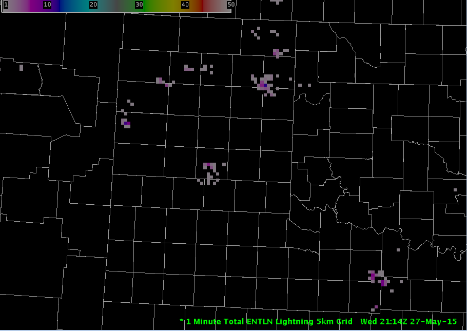
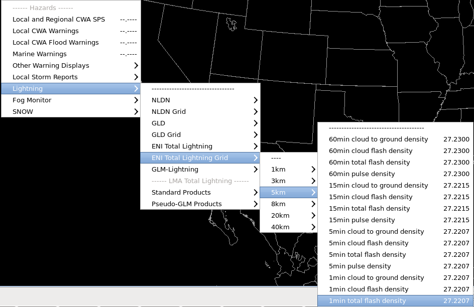
From the Obs Menu, load the 1min total flash density product on a 5km grid (alternatively you may load the 5 min plot) (Fig. 1) (Fig. 2)
-
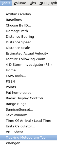
From the Tools menu, load the Tracking Meteogram Tool (Fig. 3)
-
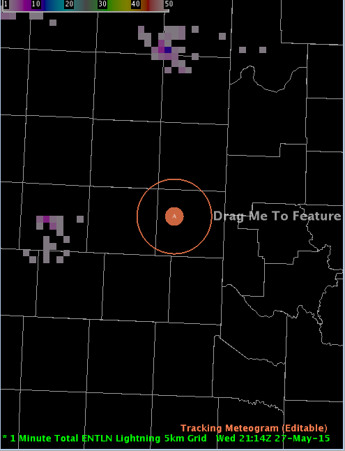
A Drag Me To Feature icon will appear. Zoom in to a location you wish to create a time series for
-
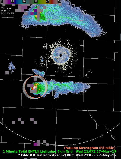
Next, confirm that you are on the last frame of data. Then resize the circle by hovering over it and using the mouse scroll wheel. Once the circle is of a desired size, drag it over the storm (Fig. 4)
-
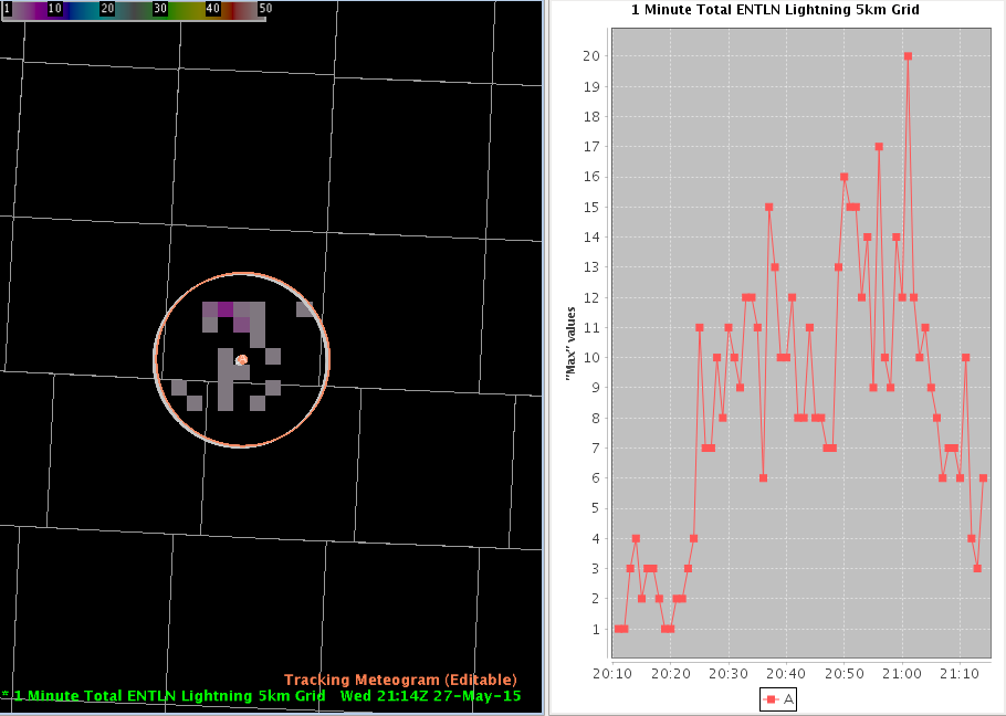
Move the circle to the point you wish to create a time series for. A time series will appear to the right of the plot (Fig. 5)
-
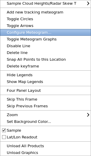
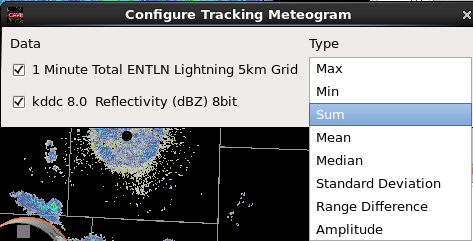
Right click and hold inside the current frame (color) circle and select Configure Meteogram (Fig. 6)
-
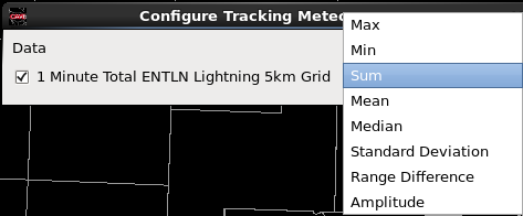
By default, the Tracking Meteogram will calculate and display the Max value inside a tracking circle. For this example we want to add up all the lightning flashes inside the circle so we will choose Sum (Fig. 7)
-
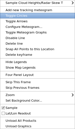
Right click and hold inside the editor and select Toggle Circles. This action removes all circles except the current frame. The result is a cleaner display (Fig. 8)
-
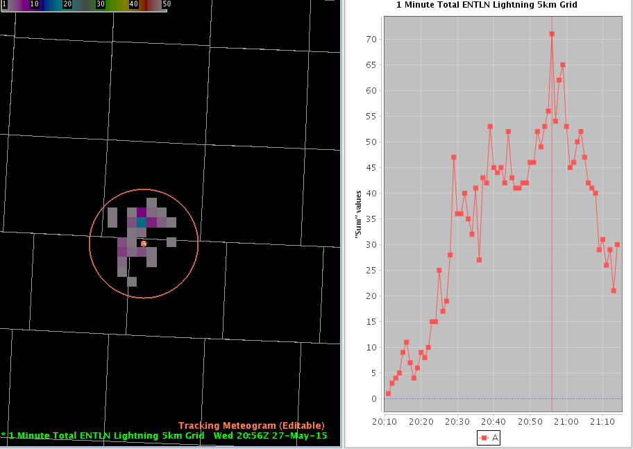
Step back to the first frame, and move that frame’s circle to the location of the feature. Step through each frame to make sure the circle captures the lightning density fields. The final display should look like this: (Fig. 9)
-
Research has shown that an increase in total lightning in a thunderstorm correlates to increased updraft strength. Thus a spike in total lightning density would suggest that the storm is trending stronger, while a decline in total lightning density would suggest the storm is weakening (although maybe just temporarily)
-
Let’s check to see if the increase in lightning density correlates with an increase in reflectivity. Load a Z product at the elevation angle which would sample the hail growth zone (environmental temperature of -20°C, -30°C, or 30-40 kft AGL would be a good place to start). In this example, I use approximately 30 kft, or the 8.0 degree elevation angle
-
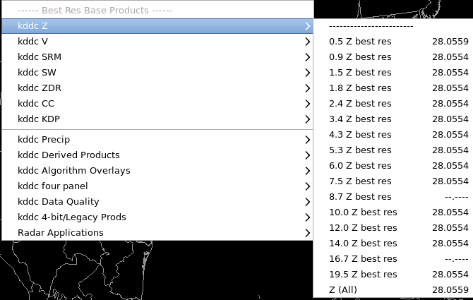
First, Clear the display. Then from your dedicated radar menu (kddc in this example), load the desired Best Res Base Product (Z) (Fig. 10)
-
Next, from the Obs Menu, load the 1min total flash density product on a 5km grid (alternatively you may load the 5 min plot) (Fig. 11)
-
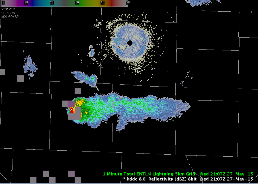
You should now see 2 stacked products displayed in the map editor: a reflectivity product and a gridded lightning density product (Fig. 12)
-
From the Tools menu, load the Tracking Meteogram Tool (Fig. 13)
-
A Drag Me To Feature icon will appear. Zoom in to a location you wish to create a time series for
-
Next, confirm that you are on the last frame of data. Then, resize the circle by hovering over it and using the mouse scroll wheel. Once the circle is of a desired size, drag it over the storm (Fig. 14)
-
Right click and hold inside the current frame (green) circle and select Configure Meteogram (Fig. 15)
-
By default, the Tracking Meteogram will calculate and display the Max value inside a tracking circle. For this example, we will keep Max for reflectivity and choose Sum for lightning density (Fig. 16)
-
Right click and hold inside the editor and select Toggle Circles. This action removes all circles except the current frame. The result is a cleaner display (Fig. 17)
-
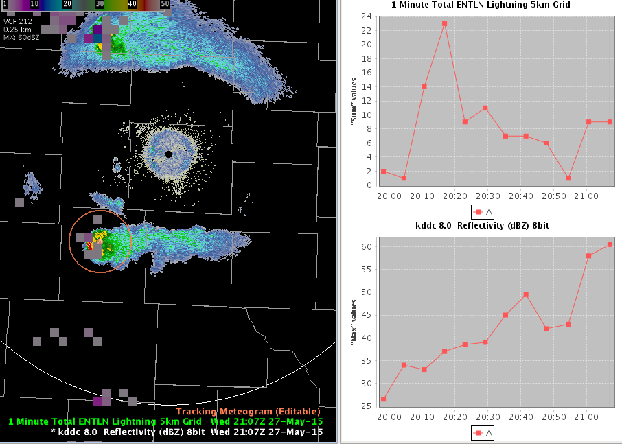
Step back to the first frame, and move that frame’s circle to the location of the feature. Step through each frame to make sure the circle captures both the reflectivity core as well as the lightning density field. The final display should look like this: (Fig. 18)
-
Looking at the time series plot, the increase in lightning from 20:05-20:15z and also from 20:50-21:05z seen on the top plot correlates with an increase in reflecivity at ~30 kft during the same time intervals on the bottom plot
Note: Resize the circle so that it captures the feature you wish to investigate without being excessively large. Huge circles can lead to undersampling of data
Note: The Tracking Meteogram does not work with Radar All Tilts, so you have to pick one elevation angle and load it separately
Note: Resize the circle so that it captures the feature you wish to investigate without being excessively large. Giant circles can lead to undersampling of data. Upgrade from 20x20 to 100x100 grid in AWIPS build 16.1.2 gives the user more room for error with circle placement. However, a region-wide circle placed over a single thunderstorm will still lead to undersampling issues even with the upgraded grid size