


TMTweb2 - OCLO
Tracking Meteogram Jobsheet 2
Purpose:
Tasks:
Jobsheet #2: Create Meteograms From a Paired Radar Product
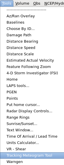
- Load a 0.5 Z+V radar paired product. Zoom to a feature you can track in Z and toggle between Z and V using the Del key on the keypad. Use the arrow keys on the keyboard to step through the Z sequence to the last frame. From the Tools menu, load the Tracking Meteogram Tool (Fig. 1)
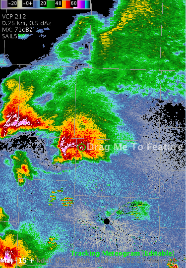
- A Drag Me To Feature icon will appear (Fig. 2)
- Move the Drag Me To Feature Icon to capture the reflectivity feature
- Enlarge the circle to the size of the feature you are tracking by hovering the mouse pointer over the circle and using the scroll wheel (Fig. 3)
- Attempt to toggle Z and V using the Del key on the keypad. This will not work, as the Tracking Meteogram breaks the functionality of this key until you click on the graph and then click on the editor (Fig. 4)
- Toggle back to Z (note you can also click on the text of the velocity product in the Product Legend to switch back to reflectivity).
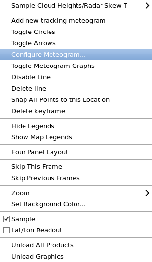
- Right click and hold inside the current frame (green) circle and select Configure Meteogram (Fig. 5)
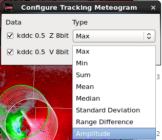
- By default, the Tracking Meteogram will calculate and display the Max value inside a tracking circle. This is fine for Reflectivity. However, suppose we want to calculate the maximum low-altitude winds associated with a mesocyclone, regardless if the Max wind is found inbound or outbound. The amplitude Type calculation will provide this.
- In the row containing the 0.5 V product, select Amplitude from the Type column (Fig. 6)
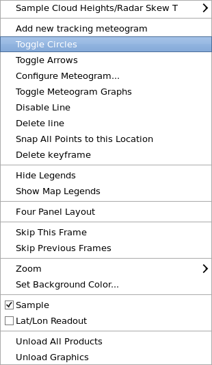
- Right click and hold inside the editor and select Toggle Circles. This action removes all circles except the current frame. The result is a cleaner display (Fig. 7)
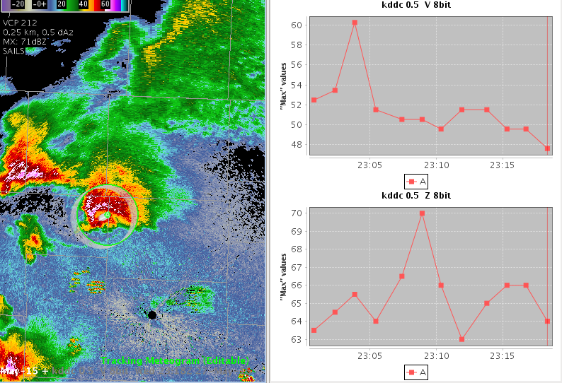
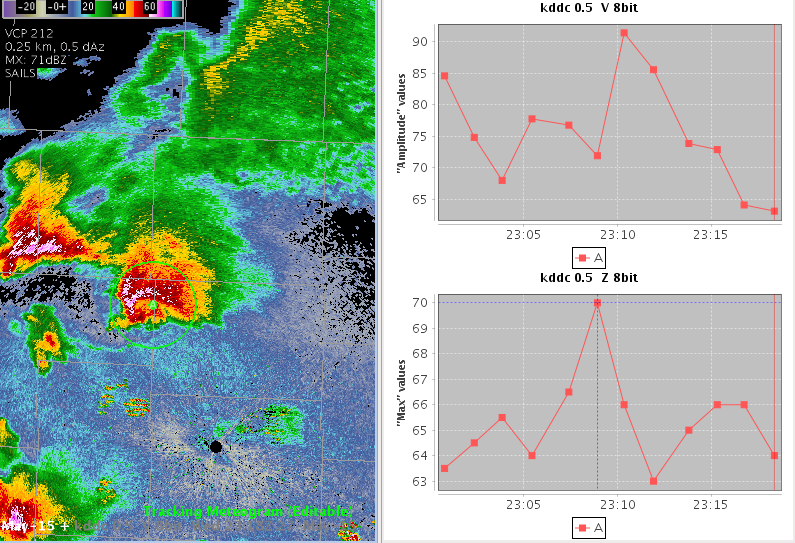
- The image below is the result of toggling off the circles and configuring the Meteogram to display Max reflectivity and Amplitude of Velocity (Fig. 8)
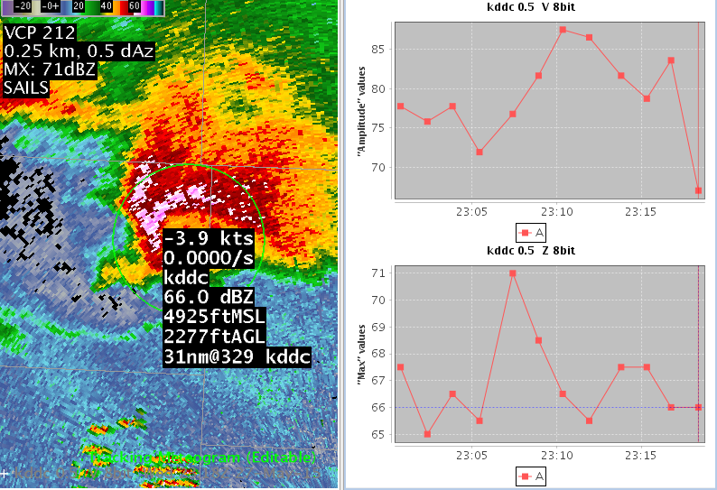
- Zoom in to the reflectivity feature you are tracking and sample the reflectivity with the mouse cursor and compare it to the Tracking Meteogram output. Change the magnification in the CAVE toolbar to a larger value, like 2.5, to be able to better read the sampled value and the ID letter at the center of the circle that corresponds to the line label in the graph (e.g. A). Use the vertical red line on the plot to identify the current frame of data. Click on the line of the data plot where it intersects the vertical red line to create the dotted horizontal blue line to aid in readout of data. The values should match or be very close (Fig. 9)
- In this example, the data is being undersampled as the Meteogram’s value of 64.5 dBZ (from the plot) is less than the CAVE sampled value of 66 dBZ. This is because the Meteogram’s 20x20 grid around the circle is too large to resolve the peak values. Thus, we need to reduce circle size to address undersampling. If your strongest Z and V values sampled are significantly different than what is plotted at the current time (note vertical red line), try reducing the size of your circle to prevent undersampling The image below shows how shrinking the circle size addresses the undersampling and results in a match (66 dBZ) between the CAVE sampled value and the Meteogram computed value (Fig. 10)
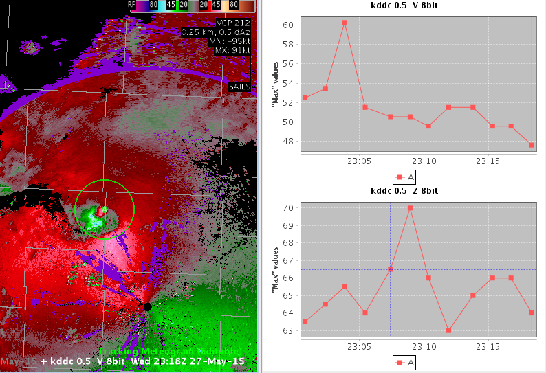
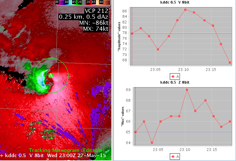
- Zoom back out, step back to the first frame, and move that frame’s circle to the location of the feature. Step through each frame to make sure the circle captures the features in Z and V. Adjust each circle’s position accordingly (Fig. 11)
- In the above example we see max reflectivities spiking to 69 dBZ and strongest velocities increasing to 86 kts
Important Tip: To recover the capability to toggle and use other keyboard shortcuts in the current map editor, left click inside the plot, and then left click back in the map editor. This will make the toggle key functional once again so you can use it to go back and forth between Z and V. Note that left clicking inside the plot will add dotted blue lines that intersect at the closest data point to where you clicked.
Note: You may have to adjust the circle position to adequately capture both max Z and strongest V in your tracking area. Go ahead and resize and reposition the circle to capture both the reflectivity max as well as the strongest velocity if needed. If the Del key toggle doesn’t work, click on the graph and then the editor.