Baselines tool

The Baselines tool, when selected, displays 10 different lines on the main display panel. These lines, labeled A-A’ to J-J’, are used to construct cross-sections from model and radar data from within the Volume Browser. These lines are “editable” by default and can be moved anywhere in the main display and adjusted to almost any length. Vertices can be added to make complex lines with a Middle-Mouse Button on the line. The Middle-Mouse Button to add vertices is a common feature to many line tools in AWIPS.

Home tool

The Home tool displays a marker (denoted with an “x” and labeled with “Home”) that is used as a reference point for displaying azimuth and range (AZ/RAN) values when sampling is enabled. The home location serves other purposes like identifying which radar the Volume Browser will use to create radar-derived graphics (nearest radar to cursor home location). The Home location is not editable by default, but can be made editable by pressing down on the scroll wheel while hovering over the Home product listing in the product menu. When editable, the Home location can be moved with a Left-Mouse Button and drag.

Choose By ID tool

The Choose By ID tool is a method to assign a point to the location of a Digital Mesocyclone Display (DMD) algorithm id by entering the id in the left-most box next to the point letter for display through the Volume Browser (not common). This tool allows the AWIPS operator to monitor the same feature over time as it moves (as long as the DMD algorithm continues to identify that feature).

Besides its use for the DMD algorithm, the Choose By ID tool can also be used to set Points, Baselines, and Home at specific locations by entering METAR, RAOB, and radar names. The left box next to the letter is for points (requires single location), and the right box is for baselines (requires two locations). You must hit the enter key to register your location entered.

Put Home Cursor tool

The Put Home Cursor tool allows the AWIPS operator to quickly identify the location of a specific METAR station, city, or Latitude/Longitude coordinate. This tool uses the Put Home Cursor GUI when the AWIPS operator specifies the method used to put Home in the new location.

Points tool

The Points tool, when selected, displays ten points in the main display panel. These points, labeled A through J, can be used to generate model soundings, vertical wind profiles (using profilers and WSR-88D VAD Wind Profiles), time-height cross-sections, time series, and variable vs. height plots in CAVE using the Volume Browser. These points are editable when loaded and can be moved to any location visible in the main display panel. You can create your own points and control their name and size separately. The points can also be launched from the button with the three dots on the CAVE toolbar.

Distance Bearing tool

The Distance Bearing tool, when selected, displays six different lines in the main display panel. Each line shows the AZ/RAN information for the labeled end of the line relative to the unlabeled end of the line. The lines are made editable by default.

Distance Speed tool

The Distance Speed tool can be used to determine the linear speed and direction of a storm or other meteorological feature by tracking a point or polyline (note vertices can be added to the line with a Middle-Mouse click). When this tool is selected, a circular marker will be displayed in the main display panel that the AWIPS-2 operator can move to the feature they wish to track. By moving the frames forward/backward to a different time, and moving the marker again to the feature, the forecaster will get a motion track with the speed or time information based on the previously edited location and the newly edited location. With "Speed" selected, the track's direction (in degrees) and speed (in knots) are displayed. With "Time" selected, the times of the beginning, end, and future position are displayed. When using the polyline mode the line must be grabbed and not the dot. Because the tool only uses two positions to create the track, an important best practice is to step multiple frames between repositioning the dot, so you won’t generate noisy, poor-quality motions. This tool works similarly to the WarnGen storm motion tool (see “WarnGen”).

Feature Following Zoom (FFZ)

The Feature Following Zoom (FFZ) tool allows a forecaster to loop a series of images that stays centered on a specific tracked feature rather than staying centered on a geographic point. The FFZ can also be used on any zoom scale. Overall, this has two primary benefits for a forecaster. One, the forecaster can perceive relative evolution more effectively with the feature always in the center of the display. Two, they can zoom in and see far greater detail throughout the loop than they could with a geographic based center for the loop.

The FFZ utilizes the Distance-Speed tool to determine where the floating center point will be located. This brings up two key points to remember when using FFZ. The first is that the most recent Distance-Speed tool or WarnGen track loaded will be used by FFZ. In other words, any update to these tools will cause FFZ to update. Second, the Distance-Speed tool only allows for linear motion, and it typically works best if the earliest and latest times in the frame sequence are used to track the feature. Non-linear motions of storms cannot be followed with FFZ.

Time of Arrival / Lead Time tool

The Time of Arrival / Lead Time tool is used to create a track for a point or line similar to the Distance Speed Tool, but it also allows the user to identify a point to calculate time of arrival. The Arrival Point can be dragged along and ahead of the track, within a circular front that expands along the track, and the time of arrival of that front is displayed.

Sunrise/Sunset

The sunrise/sunset calculator displays the times and azimuths of sunrise and sunset at a given point for a given date (either lat/lon or using cursor home). Just enter in your location/time and click the Calculate button. This can be used to explain the daily sunrise and sunset spikes in radar data.

There are a number of radar tools that directly interact with radar data loaded in D-2D, including VR-Shear, Radar Display Controls, and Estimated Actual Velocity.

VR-Shear tool

The VR-Shear tool is used in conjunction with a Radial Velocity (or Storm Relative Mean Radial Velocity Map) product to calculate Rotational Velocity and shear-related quantities. The AWIPS operator positions the two endpoints of the VR-Shear tool over the desired range gates. When positioned, the VR-Shear tool determines the Rotational Velocity (in kts), the distance between end points (in nautical miles), the shear which is the velocity difference divided by the distance between points (in s-1), and it includes the distance from the radar (in nautical miles). Rotational velocity is a very important parameter in warning-decision making, and it is calculated by taking the velocity difference between two gates across azimuths (not necessarily immediately adjacent) at similar ranges and dividing by two (e.g. 40 kt outbound and -40 kt inbound yields a 40kt rotational velocity). Note the VR-Shear tool provides rotational velocity and not velocity difference. Many expert warning forecasters find it faster and easier to sample the peak velocities in a shear signature and mentally subtracting them and dividing by two, but this tool can help you with the math if you are not used to doing that, though it can take some time to get the end points where you want.

Positive shear values measured by the tool indicate cyclonic shear, while negative shear values indicate anticyclonic shear. If either end point is not directly over a range gate with valid velocity data, the phrase “no data” will appear in place of the shear value. Shear values with small signatures over a few azimuths are extremely sensitive to noise in the data and the distance between azimuths, so rotational velocity is usually a more stable parameter in warning decision making.

NOTE: If you pan the main display panel while using the VR-Shear tool to the point where you no longer see the tool endpoints, pressing the Right-Mouse Button in the main display panel will cause the tool to snap to the point where you clicked the button. This feature is common to many of the line tools in AWIPS.

Radar Display Controls tool

The Radar Display Controls tool is a GUI that gives the AWIPS operator control over the appearance of several different radar products. The most common use of Radar Display Controls is to enter a storm motion used in the display of the SRM products to better bring out peak velocities in rotational signatures as a balanced couplet of inbound and outbound velocities.These products are managed in user override files, so the settings will follow the user when logged in to different workstations

• STI (Storm Track)
  • when displaying STI loaded from the radar menu, this filter controls how many storm tracks are shown and whether to plot the past and/or future tracks
• HI (Hail Index)
  • when displaying HI loaded from the radar menu,
    • Probability of Hail (POH) defines the % threshold used in displaying open (default 30%) and filled (default 50%) small triangles (typically superseded by POSH large triangles)
    • Probability of Severe Hail (POSH) defines the % threshold used in displaying open (default 30%) and filled (default 50%) large triangles
• TVS (Tornado Vortex Signature)
  • when displaying TVS loaded from the radar menu, "Show elevated TVS" displays elevated TVSs and is off by default due to higher false alarm rate
• DMD, MD, TVS (Digital Mesocyclone Display, Mesocyclone Display, Tornado Vortex Signature)
  • when displaying DMD, MD, or TVS loaded from the radar menu, "Show extrapolated features" allows the extrapolated features to be displayed (default is off)
• DMD (Digital Mesocyclone Display)
  • when displaying DMD loaded from the radar menu,
    • "Min feature strength" - mesocyclone clutter filter specifies the minimum 3D strength rank use to display a mesocyclone
      • default is 5 (minimal mesocyclone ~ rotational velocity [Vr] 30kts; note 3 (~20 kt Vr), 7 (~40kt Vr), and 9 (~50kt Vr)
    • "Show overlapping Mesos" toggles overlapping mesocyclones (default off)
    • Tracks pullout menu specifies whether to display past and forecast tracks
• MBA (Automated Microburst Detection Algorithm Micro-Burst Alert)
  • when displaying MBA loaded from the radar menu,
    • "Show Wind Shear" lowers the display threshold to include wind shear detections (default off)
      • wind shear 0.5 degree divergence delta-V < 23kts, area < 1.2 miles
      • microburst 0.5 degree divergence delta-V > 23kts, area < 2.5 square miles
      • macroburst 0.5 degree divergence delta-V > 23kts, area > 2.5 square miles
• SRM (Storm-Relative Mean Radial Velocity Map)
  • The motion used in the SRM display is specified in the Radar Display Controls and is displayed on the upper corner of the SRM product. Setting the storm motion subtracts out a constant from the velocities displayed in SRM to better highlight balanced peak inbound and outbound velocities in rotating storms (note that this will not impact divergence and shear calculations which are Galilean Invariant). 
    • Storm Motion from WarnGen Track - user override that applies the motion from that user's last WarnGen track or that user's last Distance Speed Tool track
    • Average Storm Motion from STI - average motion computed each volume scan from the STI product for the radar displaying SRM
    • Custom Storm Motion - user override that applies that user's last custom motion defined in the Custom Storm Motion entry using the slider bars, spin boxes, or typed in text
• SAILS 
  • "Enable SAILS Frame Coordinator"
    • toggle on (default) - keyboard shortcuts change where tilting up from 0.5 degree SAILS tilt will step to the next higher tilt (similar to GR2 Analyst) and Ctrl right arrow will step to the most recent tilt available for any elevation angle
    • toggle off - keyboard shortcuts change where tilting up from 0.5 degree SAILS tilt will not go anywhere (old confusing behavior) and Ctrl right arrow will step to the most recent time of the current tilt
  • For a summary of all-tilts keyboard shortcuts, see the All-Tilts reference page.

Estimated Actual Velocity (EAV) tool

The Estimated Actual Velocity (EAV) tool is a radar analysis tool that allows forecasters to estimate the actual wind speed based on a user defined wind direction, the measured radial velocity, and the intersection angle between the radar beam and wind direction. This tool may be useful to some forecasters during situations where a more exact wind speed is desired to include in a warning, follow-up statement, or other text product when you know the wind direction accurately (say from spotters or from surface observations in widespread damaging wind situations).

When the angle between these two vectors is relatively small (i.e., less than 45 degrees) and the forecaster has a good estimate of the actual wind direction, than this tool’s wind speed values can be more representative of what is actually occurring. When this angle is less than 20 degrees, the wind speeds returned by the tool will be similar to the radial velocity values and provide little additional benefit. When this angle is greater than 45 degrees, the equation used by the EAV tool becomes too sensitive to incremental changes in the angle to reliably determine the actual velocity.

The tool allows users to obtain the actual wind speeds in two different manners. First, the wind speed and direction are listed at either end of the line tool that forecasters use to indicate the wind direction. Second, users can access the EAV estimated velocity at any given point by using sampling which will apply the direction of the EAV tool orientation to the calculation of the velocity estimate at the sampled range gate.

When using the EAV tool, there are some guidelines you should follow:

• You should only use the EAV tool on velocity (V) data
• DO NOT use the EAV tool on Storm-Relative Velocity Map (SRM) product displays
• Only use the EAV tool in well-sampled radial velocity areas and where the wind direction is likely to be unambiguous.

More information on the EAV Tool can be found in WES Exercise 2 D2D Radar-Related Tools Estimated Actual Velocity video.

The Four-Dimensional Stormcell Investigator (FSI) has been disabled at most WFOs due to performance reasons, and is slated to be removed in build 23.4.1 when Redhat 8 is deployed. Most forecasters can skip this section.

The Four-Dimensional Stormcell Investigator (FSI) is a volumetric radar  base data display program that combines combines dynamic horizontal and vertical cross section capabilities. The FSI tool is based on the National Severe Storm Laboratory (NSSL) Warning Decision Support System - Integrated Information (WDSS-II), and is mostly separate from the CAVE and D-2D architecture. FSI is launched from D-2D after loading it from the menu, but it displays in a separate window outside of CAVE, so it cannot interact with CAVE or D-2D. 

FSI Basics

FSI allows forecasters to view a single radar’s volume scans of base data in a four-panel layout separate from CAVE. FSI is only available for dedicated radars that ingest full volume scans of data (this is changing in future builds), and some of the additional tilts, like SAILS, are filtered from the volumetric FSI display. Forecasters can view any of the four standard base data products (i.e., Reflectivity, Velocity, Storm-Relative Mean Velocity Map, and Spectrum Width) or Dual-Pol variables (Differential Reflectivity, Correlation Coefficient, Specific Differential Phase (i.e. RhoHV), and the Hydrometeor Classification (HC) one at a time, from four different displays provided in each panel. These displays are:

• Upper Left - The Plan Position Indicator (PPI), or constant vertical elevation angle, Panel;
• Upper Right - The Constant Altitude Plan Position Indicator (CAPPI) Panel;
• Lower Left - The Vertical Dynamic Cross Section (VDX) Panel; and
• Lower Right - The Three-Dimensional Flier (3DF) Panel.

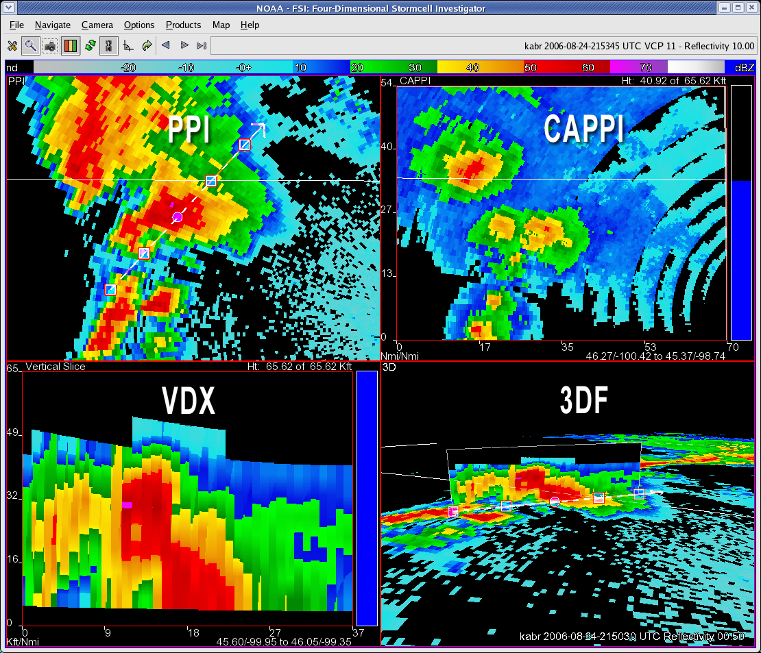
These different panels provide forecasters vantage points for dynamically analyzing the vertical and horizontal structure of base radar data. FSI is an intensive system-resource application that only allows one instance per workstation.

Loading FSI

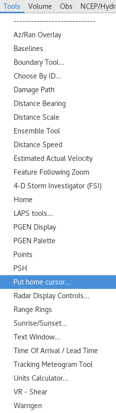
FSI can be launched from within the D-2D perspective from two different locations:

• The Tools menu
• The “Applications” section of any radar menu or “Radar Tools” menu in the Radar menu

While you are not required to load radar data before launching FSI, it is usually convenient to load radar data first to identify the location you want to launch FSI centered on.

After you initially launch the application, you will need to press the Right-Mouse Button in the editor in the vicinity of a feature you wish to interrogate. If you forget, the product legend for FSI in the main display panel reminds you of this. If your CWA has multiple dedicated radars, a radar list menu will pop up, and you will need to select the radar you want FSI to use.

Case review with FSI in WES-2 Bridge requires unique data handling, and popup messages will warn you when you can select a radar to launch FSI with after WES-2 Bridge is done creating the data. This is not an issue with running a simulation in WES-2 Bridge.

Using FSI

FSI displays data from any base moment and variable, but the same product appears in all four display panels simultaneously. The displays are linked so that when the user toggles a new product, zooms, or pans in one display, all of the other displays will update accordingly. Users can toggle between radar base products by using the following keyboard shortcuts from the main typing area of the keyboard (i.e., not the numeric keypad):

• Base Reflectivity - “Z” or “1”
• Base Velocity - “V” or “2”
• Storm-Relative Velocity Map (SRM) - “S” or “3”
• Spectrum Width - “W” or “4”
• Differential Reflectivity - “D” or “5”
• Correlation Coefficient - “O” or “6”
• Specific Differential Phase - “K” or “7”
• Hydrometeor Classification Algorithm - “H” or “8”

The following sections provide a brief overview of each display panel, the general uses for both the menu bar and button panel items, and some other important points about FSI to know prior to working on the WES Exercise 4 D2D Four-Dimensional Stormcell Investigator Basics video.

The PPI Panel (upper left)

The PPI Panel displays an elevation-based radar product similar to what you’ve seen in D2D base data displays. Users can toggle up-and-down in elevation or back-and-forth in time to change the appearance of this display panel using the menu bar, button panel, or numeric keypad (more details on how to perform these tasks in Sections v-vii).

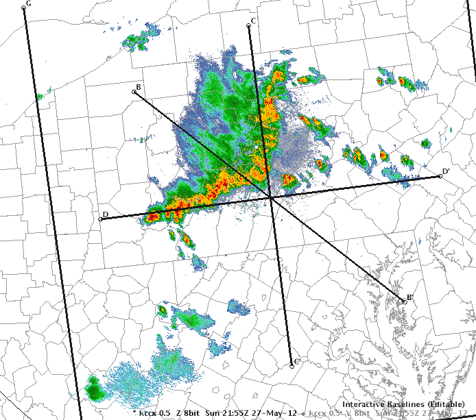
In addition to the base data, the PPI Panel contains the vertical cross-section control tool. This tool is a dashed white line with five points that indicate and control the position of the vertical cross-section axis displayed in the VDX panel. You can press and hold on one of these points of the cross-section to dynamically adjust the image in the VDX display using the following controls:

• The circle at the middle of the cross-section allows the user to adjust the horizontal position of the entire axis;
• The square points at either end of the cross-section allows the user to adjust the end points of cross-section; and
• The square points between the end and center of the cross-section allow the user to rotate the axis around the center point of the line.

The CAPPI Panel (upper right)

The CAPPI Panel allows forecasters to quickly visualize base moment data at a constant elevation which can be useful for comparing storms at different ranges. FSI allows forecasters to display CAPPIs and change their MSL height quickly. To adjust the height above MSL (AGL heights are not available in FSI) of the CAPPI, use the blue vertical bar immediately to the right of the display panel.

The VDX Panel (lower left)

The VDX Panel shows a vertical cross-section of base data represented by the vertical cross-section control tool in the PPI and 3DF Panels. Changing the location, length, or orientation of the cross-section axis in either of the previously mentioned panels will result in the VDX Panel updating dynamically. In addition to altering the display with the vertical cross-section control tool, users can adjust the vertical scale of the cross-section by using the blue vertical bar immediately to the right of the display panel.

The 3DF Panel (lower right)

The 3DF Panel plots both the vertical cross-section and either the PPI or CAPPI displays in true 3-D earth coordinates. As in the PPI Panel, the vertical cross-section tool is visible in the 3DF Panel and can be used to dynamically adjust the display in the VDX Panel using the same controls as mentioned previously in the PPI Panel. The 3DF Panel allows forecasters to visualize WSR-88D volumetric data on a single display. Novice forecasters who are not familiar with viewing three-dimensional radar visualization products may require some time to become confident at interpreting data in the 3DF Panel.

Menu bar

The menu bar contains several menus:

• File - Used primarily for saving current or restoring default settings as well as to exit the FSI extension
• Navigate - Contains a complete list of traditional volume navigation and some alternative volume browsing hot keys
• Camera - Contains a list of some alternative display navigation hot keys
• Options - Contains a list of additional display option hot keys
• Products - Contains a list of product selection hot keys
• Map - Map overlays can be added, hidden, removed, or configured here for all of the display panels
• Help - Contains an about screen for FSI

Button panel

The Button Panel contains several features that can be accessed by selecting the following buttons:

• Preferences - Used to open the “Edit Preferences” pop-up window
• Readout (Data Sampling) - Toggles data sampling on/off
• Snapshot - Opens the “Take Snapshot” pop-up window to make image captures of FSI
• Color Key - Toggles the color key off/on under the FSI Button Panel
• Loop - Toggles looping on/off (NOTE: Loop preferences are editing using the “Edit Preferences” pop-up window)
• Auto-Update - Toggles automatic radar data updates on/off
• Plan View - Resets the viewing angle of the 3DF Panel to the default position
• Reset - Restores the FSI Extension panels to the initial conditions of when you last launched FSI
• Back - Steps the display panels back one volume scan while maintaining the current elevation angle
• Next - Steps the display panels forward one volume scan while maintaining the current elevation angle
• Latest - Steps the display panels forward to the current (or latest volume scan available) while maintaining a constant elevation angle
• Radar Status Bar - Continuously updating readout showing the date, time, VCP, and elevation angle of the most recently completed elevation scan from the radar and the product being viewed

Basic panel controls

These mouse-based control features are:

• Zoom - Press and hold the Middle-Mouse Button while moving the mouse forward (zoom in) or backward (zoom out). Alternatively, roll up (down) on the scroll wheel to zoom in (out).
• Pan - Press and hold the Left-Mouse Button while moving the mouse to “pull” the image to the desired location
• 3D Rotate- With the mouse cursor over the 3DF panel, press and hold the Left-Mouse Button and <SHIFT> key while moving the mouse forward (increase viewing angle) or backward (decrease viewing angle) to adjust the viewing angle in the 3DF Panel

The numeric keypad is the easiest way to navigate through the radar volumes and alter the camera views (note the D2D All Tilts navigation arrows do not work with FSI). The numeric-keypad controls are (NOTE: For the following commands to work, you will need to have “Num Lock” toggled on):

• “8” Key - Move up one elevation angle in traditional volume scan
• “2” Key - Move down one elevation angle in traditional volume scan
• “4” Key - Move backward one volume scan at constant elevation angle
• “6” Key - Move forward one volume scan at constant elevation angle
• “9” Key - Move up one elevation angle in virtual volume scan
• “3” Key - Move down one elevation angle in virtual volume scan
• “.” Key - Toggle between Reflectivity and Storm-Relative Velocity Map products
• “+” Key - Zoom camera view in
• “-” Key - Zoom camera view out
• “/” Key - Tilt camera view up in 3DF Panel
• “*” Key - Tilt camera view down in 3DF Panel

Other Important Issues with FSI

In addition to all of the previous features and controls discussed, there are a handful of other important items to mention related to FSI. These items are:

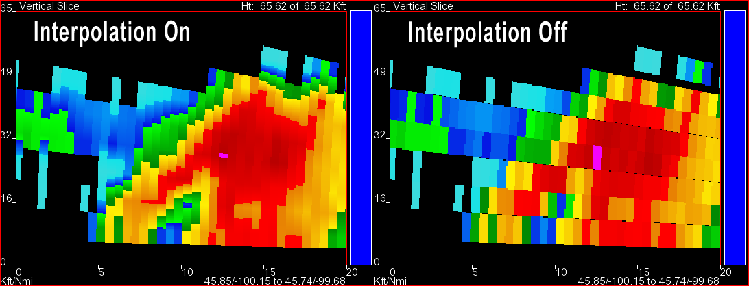
Interpolation

FSI allows users to toggle on data interpolation for the CAPPI, VDX, and 3DF Panels. This interpolation feature is turned on by default. Interpolation can be toggled using the “I” keyboard shortcut or by using the Options menu to be able to visualize radar sampling limitations of gaps between beams. More on the interpolation feature will be discussed in the WES Exercise 4 D2D Four-Dimensional Stormcell Investigator Basics video.

City name labels

FSI allows the user to add various map overlays to all of the display panels. One of these overlays (Cities --> NAME) has been shown to severely limit the performance of FSI. We strongly recommended not using the Cities--> NAME overlay in FSI.

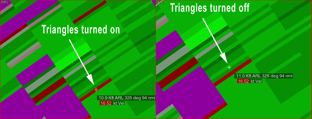
Using triangles for more accurate sampling

While you have to ability to toggle sampling on, the accuracy of that sampling will vary depending on one of your settings in the “Edit Preferences” window. That setting, called “Use Triangles over Textures” (found under Advanced Settings --> Display --> OpenGL), will result in more accurate sampling when turned on and is recommended. However, there is a reduction in performance when this option is turned on. More on this issue with sampling will be discussed in the WES Exercise 4 D2D Four-Dimensional Stormcell Investigator Basics video.

Virtual volume scan

FSI renders the latest volume scan as a 3D cube prior to all the data being collected. It does this by using the previous volume scan as a first guess and updating the tilts as they come in. Thus, while data is arriving on the current volume scan, there will be a discontinuity as the old data is routinely replaced with the new data.

TDWR in FSI

TDWR data can be displayed in FSI if there is a TDWR in or near a forecaster’s CWA. The primary advantage of TDWR in FSI is volumetric analysis using dynamic vertical and horizontal cross-sections. However, there are a few caveats you must remember when viewing TDWR in FSI:

• Some tilts are omitted to allow FSI to display the data
  • Long-range reflectivity
  • Four of the 0.5 degree scans
• First tilt of second sub-volume is adjusted in time
• Large data gaps in vertical can hinder volumetric analysis (use interpolation)

As a final reminder, D-2D will continue to display all of the TDWR data, so if a forecaster wants to continue to use all the TDWR data available, they will have to use D-2D. However, if a forecaster is interested in volumetric analysis of TDWR data (e.g. vertical cross sections), that can be done now in FSI.

To see FSI in action, see this previous training video.

The Damage Path Tool (DPT) is a D-2D tool that is used to provide first responders with near real-time damage polygons containing comments. After loading the Damage Path Tool from the D-2D Tools menu, the user creates a polygon using a polygon editing tool similar to WarnGen or using a special tornado track tool. With the tornado track tool, the user modifies a D-2D baseline along the track of a tornado vortex signature, and the tool creates a tornado track with a width that is a function of the radar tornado location uncertainty that increases with range from the radar. With uncertainties of ~ 0.5 mile at 40 nmi and ~ 1 mile at 80 nmi, the tornado path width varies from 1 mile at 40 nmi to 2 miles at 80nmi to account for radar range-dependent uncertainty in radar vortex location and actual tornado damage location at the surface.

After the user creates a polygon, a right mouse click on the polygon is used to launch the Set Properties dialog which is used to specify information about the damage. The DPT supports the following damage types:

Preliminary Tornado

Significant Wind Damage

Hail

Flood

Extreme Ice or Snow

Other Man Made/Natural Hazard

After creating the polygon and inputting damage metadata, the user can right click on the damage path to export to a GeoJSON file that can be posted to the web or emailed to local first responders. The DPT also has a right click option to send the damage path to the Damage Assessment Toolkit server where first FEMA and first responders can get access to the data.

There is no directive on the DPT use, and a significant amount of preparation needs to happen before an office would consider issuing polygons. The situations where an office will choose to use it need to be defined and coordinated with local stakeholders to ensure they are prepared to use this type of information. While the DPT was originally designed for use for providing near real-time significant tornado damage paths in rare high-impact situations, it supports a wide variety of decision support situations. For more on the DPT, see the Damage Path Tool training in the CLC and the DPT VLab reference page.

The Tracking Meteogram Tool (TMT) allows the user to track meteorological features using circles on each frame of data to create time trend plots of the data loaded. The TMT is loaded from the Tools menu and utilizes the familiar Drag Me to Feature icon to track a desired feature through space and time. Once loaded, the user interacts with the TMT by right clicking on the circle or graph to configure its properties.

The tool is compatible with any gridded image data including: satellite, radar, model, and total lightning density. It utilizes a 100x100 grid box that encompasses a tracking circle that the AWIPS operator can position over the data. The tool performs calculations inside the circles based on the math operation specified by the AWIPS operator (max, min, sum, mean, median, standard deviation, range difference, and amplitude). In addition to tracking features in space, the Tracking Meteogram Tool can also monitor data at a single point by snapping all circles to a single location.There are a few limitations to using the tool, including: breaking of keyboard shortcuts, non-functionality with all-tilts data, and inability to save settings like graph colors and fonts in procedures.

The Tracking Meteogram Tool will not be used in RAC, but if you would like to learn more about it, see the training in the CLC and the Tracking Meteogram Tool VLab reference page for the accompanying reference and job sheets.

The Ensemble Tool is designed to create new display fields from gridded ensemble datasets (mean, min, max, median, range, sum, and standard deviation) and to facilitate cycling through multiple model family displays. There are two important tabs. The Legends tab and the Matrix tab.

Legends Tab

The GFS Ensemble Forecast System (GEFS) is the primary ensemble dataset available in AWIPS for use with the Ensemble Tool at WFOs. The AWIPS GEFS dataset contains a 21-member ensemble of surface temperature and precipitation, as well as a 12-member ensemble of Mean Sea-Level Pressure, max temperature, min temperature, and a wide variety of fields (height, temperature, relative humidity, and wind) at standard pressure levels (1000mb, 925mb, 850mb, 700mb, 500mb, and 250mb).

To use the Ensemble Tool to create new derived field displays, the user first loads the tool from the Tools menu and then uses the Volume Browser to load a parameter in the ensemble dataset. Each member loads as a separate color that can be toggled on or off, and the user clicks the gear button to choose what field will be calculated for the visible members toggled on. For example, to compute the minimum value at each point among all the members, the user selects Min. The minimum value is then computed and added as a contoured image in the display. Derived fields cannot be converted to images, however. The derived fields do allow for specific contour control that is unique to this tool.

The Ensemble Tool also allows for sampling of all the fields in the display, and it also contains a distribution viewer (also accessible from the gear menu) for creating probability density function/cumulative density function graphs. After loading the distribution viewer, as the user samples the display, the distribution graph of all the members updates for the location of the mouse pointer.

In the distribution graph, each ensemble member value is indicated by a red tic mark on the x axis. The range of data is broken up into bins and the number of values in the bins is plotted along with the cumulative percentage at and below the values. This can be particularly useful in diagnosing different solution modes, say for when half the members have large precip and half have none and an average value can be misleading. 

Matrix Tab

The Matrix tab of the Ensemble Tool allows the user to load groups of model family parameters available from the Volume menu and rapidly cycle through the different models. The are different model family presets that can be selected from the initial menu upon clicking on the Matrix tab, each tailored for use in different meteorological scenarios (winter, severe weather, etc.). While you can combine different models in a four panel display, the Matrix tab within the Ensemble Tool is a more dynamic and relatively easy way to load and cycle through multiple models at different times. In 17.3.1, the Matrix tab will have problems that will be fixed in 18.1.1.

The Ensemble Tool will not be used in RAC, but if you would like to learn more about it, see the Ensemble Tool VLab reference page with job sheets.

The Boundary Tool was designed for the Aviation Weather Center to track boundaries, and users can create boundary overlays that can persist in time up to 8 hours. The boundary tool uses a familiar-looking distance speed line tool that is overlaid on a feature to be tracked. These boundaries cannot be shared, though they can be saved and reloaded. While this tool can be used by others than the Aviation Weather Center, it is sensitive to the order of certain commands and can take some time to get used to.

The Boundary Tool will not be used in RAC, but if you would like to learn more about it, see the Boundary Tool VLab reference page and associated job sheets.

There are a few other D-2D tools worth mentioning, including Text Window, PGEN, LAPS tools, Units Calculator, and WarnGen. 

Text Window

While on an operational AWIPS you typically have the text workstation loaded on a separate monitor from CAVE, you can additionally load a text window from the Tools menu if you want to view a text product from the database.

Product Generator (PGEN)

The National Centers use PGEN to draw annotations and generate all their products, and it is included in D-2D to support Center Weather Service Units (CWSUs) making AWC-style SIGMETs. While this is not intended to be used for other purposes, there are a number of unique drawing and annotation tools that can be used to make images using the CAVE->export->Image once a display has been created. "PGEN Palette" under the Tools menu can be  used to draw, annotate, and open/save displays. "PGEN Display" under the Tools menu can only be used to retrieve saved PGEN sessions.

Local Analysis and Prediction System (LAPS) Tools

There is a LAPS tool for the LAPS focal point to identify what data was ingested in the LAPS objective analysis and to view and redefine the LAPS analysis domain.

Unit Calculator

If you ever need to convert units in D-2D, you can use the Units Calculator from the Tools menu. Just select the desired unit checkboxes, enter a number, and hit enter.

WarnGen

You can load WarnGen from the Tools menu or the D-2D yellow button on the toolbar.