


Tilt Apparent Vertical Profile of Reflectivity - Warning Decision Training Division (WDTD)
Navigation Links
Products Guide
Tilt Apparent Vertical Profile of Reflectivity
Short Description
Algorithm that corrects for bright band contamination in reflectivity data prior to its use in the Seamless Hybrid Scan Reflectivity (SHSR) for calculating Surface Precipitation Rates (SPRs).
Subproducts
None.
Primary Users
None. This data is primarily used as an input for the Seamless Hybrid Scan Reflectivity product that feeds the Surface Precipitation Rate product within and above the melting layer.
Input Sources
Radar Reflectivity, NOAA/NCEP Rapid Refresh (RAP) with nested High-Resolution Rapid Refresh (HRRR) temperature sounding at each radar site
Resolution
Spatial Resolution: one file per radar
Temporal Resolution: 5 minutes (i.e., per volume scan)
Product Creation
The Tilt Apparent Vertical Profile of Reflectivity (Tilt AVPR) algorithm is used to identify bright band (BB) contamination in single site base reflectivity radar data, and to correct for it in affected stratiform regions and ice regions, prior to its use in the Seamless Hybrid Scan Reflectivity (SHSR). To accomplish this, the algorithm identifies stratiform regions that may have a bright band. For each radar elevation scan, the Tilt AVPR is calculated by taking the 360° azimuthal average of reflectivities at each constant range within the BB area. Using the Tilt AVPR, the BB top, bottom, and peak are determined, and a model is fitted to the AVPR that determines appropriate slopes and makes one continuous profile. This “idealized” Vertical Profile of Reflectivity (VPR) is the final step for creating the stand-alone Tilt AVPR product.
To complete the correction algorithm, the observed reflectivity (at a particular height) is compared to the idealized VPR at that height, and the observed reflectivity is corrected. These corrections are only made in ranges where the idealized AVPR was calculated (i.e. beyond the range of the BB bottom). Further, the corrections are only applied in: 1) the BB areas between the ranges of the BB top and bottom, and 2) the stratiform areas beyond the BB top (i.e. in the ice region). It should be noted that the VPR in the ice region is calculated using all azimuths, as long as there is stratiform precipitation beyond the BB top.
Technical Details
In radar meteorology, the “bright band” (BB) refers to a layer of locally higher reflectivity values associated with the melting of frozen hydro-meteors (e.g. hail or aggregated snow). Quantitative Precipitation Estimate (QPE) calculations made when the radar beam is within the bright band are subject to over-estimates as the water-coated hydrometeors backscatter power more efficiently (because they look like really big drops), resulting in higher reflectivity values. However, above the bright band, reflectivities are generally lower due to frozen precipitation, in general, being less efficient in backscattering radiation to the radar. Therefore, if the beam is far enough in range that it is well above the freezing level (and thus, sampling in the ice region), then QPE under-estimates can occur. At this distance from the radar, the sampled particles are frozen (i.e., lower returns); but by the time they hit the ground, they have passed back through the melting layer and are liquid.
The following steps are used to correct for bright band contamination:
- Classify the reflectivity as either convective or stratiform using the Convective/Stratiform Precipitation Separation (CSPS) algorithm described in its documentation.
- Blockage must be less than 50% for a bin to be considered.
- Further divide the stratiform region into areas affected by the BB and those that are not. This is based on the location of the BB top and bottom, as well as exceeding a predefined composite reflectivity threshold.
- The algorithm estimates a first guess bright band area (Zhang and Qi, 2010), such that:
- BB_top = freezing level height (from RAP model analysis) + D1
- where D1 = difference between the height of the center and the height of the bottom of the lowest beam that intersects the freezing level (i.e. 3-dB beamwidth)
- BB_bottom = BB_top – 5 km
- Exceed a composite reflectivity of 30 dBZ (default).
- BB_top = freezing level height (from RAP model analysis) + D1
- The Apparent Vertical Profile of Reflectivity (AVPR) correction is only applied to the BB-affected area. This reduces the opportunity of over-correcting in non-BB areas, or under-correcting in BB areas (as might occur if using a mean Vertical Profile of Reflectivity).
- The algorithm estimates a first guess bright band area (Zhang and Qi, 2010), such that:
- For each radar elevation scan, the Tilt AVPR is calculated by taking the 360° azimuthal average of reflectivities at each constant range within the BB area.
- A mean observed reflectivity is calculated at a given range (height) when there are sufficient BB-area pixels at that range (blue dots in Figure 1).
- The minimum number of pixels is a function of range, since the beam broadens with range, thus, there are less pixels the farther out from the radar.
- A running average in the vertical is applied to the AVPR, and any points that strongly deviate from that average are tossed. If there are too many bad points (> 40%), then the VPR is tossed. When this occurs, no corrections are done.
- NOTE: For each radar range bin beyond the bright band top, “stratiform” classified reflectivities > 0 dBZ are azimuthal averaged; this constitutes the AVPRs within the ice region and will be used to create the idealized VPR (Zhang et al., 2012).
- A mean observed reflectivity is calculated at a given range (height) when there are sufficient BB-area pixels at that range (blue dots in Figure 1).
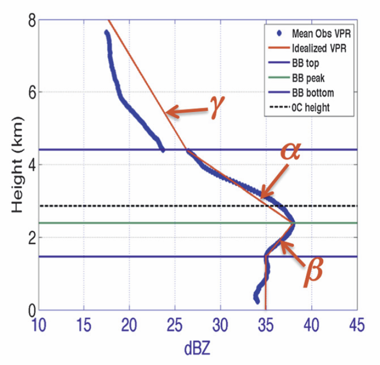
- The bright band peak (green line in Figure 1) is identified within a radar’s AVPR by finding the local maximum reflectivity closest to the freezing level (dotted line in Figure 1). The final BB top (bottom) is defined as the first AVPR inflexion point above (below) the BB peak.
- Once the BB top, bottom, and peak are determined (see Figure 1), a least squares linear model is fitted to the AVPR data using the three levels. Specifically, the model is applied to the AVPR profile to create idealized slopes between:
- the bright band top and the ice region (γ in Figure 1)
- the bright band top and the bright band peak (α in Figure 1)
- the bright band peak and the bright band bottom (β in Figure 1)
- These slopes determine the amount of corrections made to the observations. They are connected to make one continuous idealized VPR (red line in Figure 2).
- This is the final step for creating the stand-alone Tilt AVPR products. Figure 4 is a real-time example of Tilt AVPRs from multiple tilts at a radar site (KLWX). Both the azimuthally-averaged (Step 3) and idealized curves (Step 4-6) represent Tilt AVPRs, and are provided in the final product.
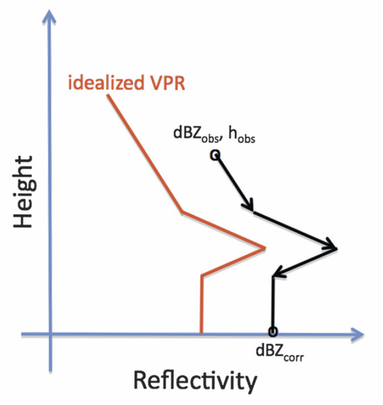
- To complete the correction algorithm, the observed reflectivity (at a particular height) is compared to the idealized VPR at that height, and the observed reflectivity is corrected based on the following relationship:
where ‘h’ is the radar beam center height, ‘ho’ the BB bottom height, ‘dBZobs’ the observed reflectivity, ‘dBZcorr’ the reflectivity after the correction, and ‘dBZAVPR’ the reflectivity in the linearized AVPR used to correct dBZobs. Figure 2 shows this VPR correction process, and how the adjustments affect the corresponding values for rainfall estimation at the surface.
- When the radar beam center is within the bright band, dBZAVPR(h) – dBZAVPR(ho) is a positive value. Hence, the corrected reflectivity is lower than the observed (i.e. lowering the overestimation).
- If the radar beam is high enough above the bright band top, the same quantity becomes a negative value; hence, the corrected reflectivity is higher than the observed (i.e. increasing the underestimation). This is the case in Figure 2.
8. These corrections are only made in ranges where the idealized AVPR was calculated (i.e. beyond the range of the BB bottom). Further, the corrections are only applied in: 1) the BB areas between the ranges of the BB top and bottom, and 2) the stratiform areas beyond the BB top (i.e. in the ice region). It should be noted that the VPR in the ice region is calculated using all azimuths, as long as there is stratiform precipitation beyond the BB top.
References
Zhang, Jian, and Youcun Qi. "A real-time algorithm for the correction of brightband effects in radar-derived QPE." Journal of Hydrometeorology 11.5 (2010): 1157-1171.
Zhang, Jian, et al. "Radar-based quantitative precipitation estimation for the cool season in complex terrain: Case studies from the NOAA Hydrometeorology Testbed." Journal of Hydrometeorology 13.6 (2012): 1836-1854.
Zhang, J., K. Howard, S. Vasiloff, C. Langston, B. Kaney, Y. Qi, L. Tang, H. Grams, D. Kitzmiller, J. Levit, 2014: Initial Operating Capabilities of Quantitative Precipitation Estimation in the Multi-Radar Multi-Sensor System. 28th Conf. on Hydrology, Amer. Meteor. Soc.
Convective/Stratiform Precipitation Separation documentation
Other MRMS product documentation: Seamless Hybrid Scan Reflectivity
Applications
The Tilt AVPR is the basis of the AVPR Correction Algorithm that corrects for bright band contamination prior to its use in the Seamless Hybrid Scan Reflectivity (SHSR) product. Properly accounting for the bright band can help create more accurate Surface Precipitation Rates (SPRs), which ultimately lead to more accurate quantitative precipitation estimates (QPEs).
Example Images
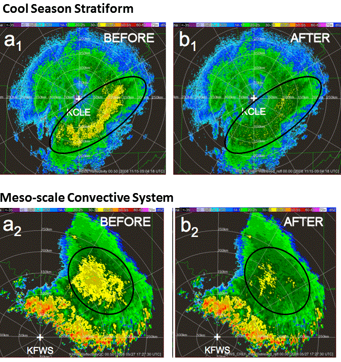
Figure 3. Examples of reflectivity data before and after the AVPR correction process. Black ovals denote the areas of reflectivity changed by the AVPR correction. (a1, b1) cool season stratiform BB contamination and correction, and (a2, b2) mesoscale convective system BB contamination and correction.
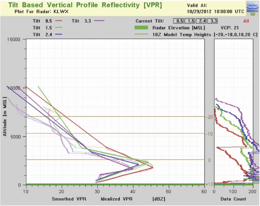
Figure 4. Tilt AVPRs from KLWX radar at 10:00 UTC on October 29, 2012. Colored curves in the main panel show profiles of azimuthally-averaged reflectivities from the stratiform precipitation areas of different tilts. The straight lines are the linear-fitted AVPRs. Curves in the right panel show number of data samples associated with the azimuthal mean reflectivities at each height.(Image from Zhang et al. 2014)