Probability of Warm Rain (POWR) - Warning Decision Training Division (WDTD)
Navigation Links
Products Guide
Probability of Warm Rain (POWR)
Short Description
Identifies reflectivity areas with potentially high (enhanced) precipitation rates using decision tree logic based on environmental predictors from the model analysis.
Subproducts
None.
Primary Users
NWS: WFO, RFC
Input Sources
NOAA/NCEP Rapid Refresh (RAP) with nested High-Resolution Rapid Refresh (HRRR) hourly environmental analysis
(The HRRR is used within its domain. The RAP is used everywhere else, which mostly affects basins near or within Canada.)
Resolution
Spatial resolution: 10 km x 10 km
Temporal resolution: 60 minutes
Product Creation
The Probability of Warm Rain (POWR) finds areas where enhanced warm rain processes and potentially high rain rates can be occurring. POWR is based on the idea that warm rain enhancement of rain rates is underestimated by current Z-R relationships; thus, the goal of POWR is to relay confidence in radar QPE underestimation at each point. The focus of the POWR is to determine the airmass properties that define these areas dominated by warm rain processes. Therefore, 19 environmental parameters from the hourly HRRR (or RAP) model (related to moisture content, instability, and temperature) are incorporated into the calculations.
First, a model “training period” determines parameter thresholds to define the ensemble of decision trees that will classify a grid point as either “underestimated” radar QPE or “overestimated”. In real-time, the same parameters are collected based on storm-relative inflow upstream of each grid point. The parameters are run through the ensemble, and at the end of each decision tree, the point is classified. The final POWR value is the proportion of decision trees that labeled the point “underestimated”. Therefore, a POWR value greater than 50% denotes that the majority of scenarios believe that the grid point has underestimated radar QPE.
Through this process, several RAP parameters were determined to have a significant impact on the results. The key predictors are 1000-700 mb mean relative humidity, 850-500 mb lapse rate of temperature, and height of the freezing level. Weak updrafts (i.e. weak lapse rates), high freezing levels (i.e. deep warm layer for warm rain growth), and high relative humidity in low/mid-levels (i.e. reduced evaporation of drops and/or low cloud bases) were found to play a big role in the occurrence of enhanced warm rain, because the residence time of drops in the warm cloud layer is prolonged, and thus, create larger drops.
Technical Details
Latest Update: MRMS Version 11
Accessible on: MRMS Development site
Methodology of the training process
Since the POWR needs to be used throughout the CONUS at any time of the year, single thresholds of each parameter may not be sufficient for such a broad range of storm modes and environmental conditions. Instead, the POWR uses a statistical machine learning method that has a “training” period to teach the model about the environmental predictors. The algorithm attempts to retrieve model environmental data upstream from a grid point (i.e. from the inflow), in hopes that any ongoing convection at the grid point will not affect the environmental variables (for all but the larger mesoscale convective systems). During the training period, 100 decision trees are created with different combinations of parameter thresholds that incorporate multiple event types in different geographic regions.
For each decision tree, a random sample of rain gauges are collected, and the radar rainfall bias are calculated by comparing the radar QPE value (using the convective Z-R relationship) at the gauge site against its collocated hourly gauge accumulation. Only the sign (positive or negative) of the bias is recorded, so a grid point will either be classified as “radar QPE overestimated” or “radar QPE underestimated”. The reason for this binary classification is because the goal of POWR is to relay a confidence in predicting radar QPE underestimation, not matter the magnitude. If it is found that the Z-R relationship underestimates the rainfall, this result denotes that there should be higher rainfall values at this location, and thus, potentially higher rain rates and warm rain processes.
At the start of each decision tree, the entire random sample of rain gauges is fed into a Classification and Regression Tree (CART) algorithm (Figure 1). At each gauge site, the associated environmental values are collected based on storm-relative inflow upstream from the site. The algorithm then decides which of the 19 environmental parameters best splits the gauges by their two bias classifications (underestimated or overestimated). This is done by finding the threshold of that parameter that best describes the bifurcation (Step 1 in Figure 1). For example, the algorithm might find that a model surface temperature of 15°C is the parameter and threshold combination that best divides the gauges by their bias classification (e.g. underestimated gauges have a surface temperature below 15°C within their inflow environment).
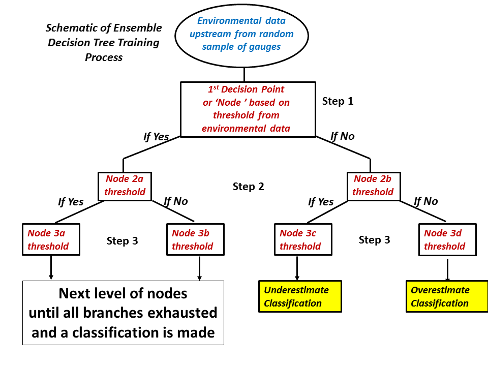
Once the parameter and its threshold are determined, the gauges are split based on whether they exceed that threshold. Those gauges with environments that do meet the criteria are then met with another parameter selection (Step 2, Node 2a). Of the remaining 18 parameters and the subset of gauges, a new parameter and threshold are determined that best explains the bias classification. The same is done for those gauges that do not meet the original criteria (Step 2, Node 2b); they are also faced with their own parameter and threshold selection (which does not have to be the same as the gauges that met the criteria).
These environmental parameter selections are continued until either: a) all gauges are classified as underestimated or overestimated (Step 3, Node 3c and 3d), or b) the subset of gauges to make the selection drops below 10. Once the decision tree is complete, the organization of it (i.e. the level a parameter is used, and its determined threshold) is saved. This process was completed for 100 different decision trees to create an ensemble. The trees varied because the random sample of gauges that forced the decision trees varied. These 100 trees made up the “training” process (which was only completed once), and from now on, the ensemble is used to create the POWR.
Methodology of the real-time product
While the training process used gauge sites where observations were available for comparison, the real-time version uses the ensemble developed in the training to create a probability at each grid point in the domain. The algorithm again collects data for the 19 environmental parameters that make up the inflow of the grid point; then, the data is subject to the ensemble of decision trees. The final result from the ensemble at the grid point is 100 classifications of either “underestimated” or “overestimated”, based on how the grid point’s inflow parameter values are classified through each of the 100 decision trees. Finally, the Probability of Warm Rain at the grid point is determined by the number of decision trees that gave the grid point an “underestimated” classification:
POWR = (total number of decision trees indicating an underestimate) / (total number of decision trees)
For example, if 90 of the 100 decision trees gave the grid point an “underestimated” classification, then the POWR at that point is 0.90.
References
Grams, Heather M., Jian Zhang, and Kimberly L. Elmore. "Automated Identification of Enhanced Rainfall Rates Using the Near-Storm Environment for Radar Precipitation Estimates." Journal of Hydrometeorology 2014 (2014).
Tropical Rain Identification documentation
Other MRMS product documentation: Surface Precipitation Type, Surface Precipitation Rate
Applications
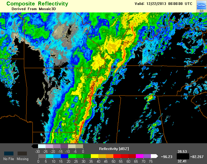
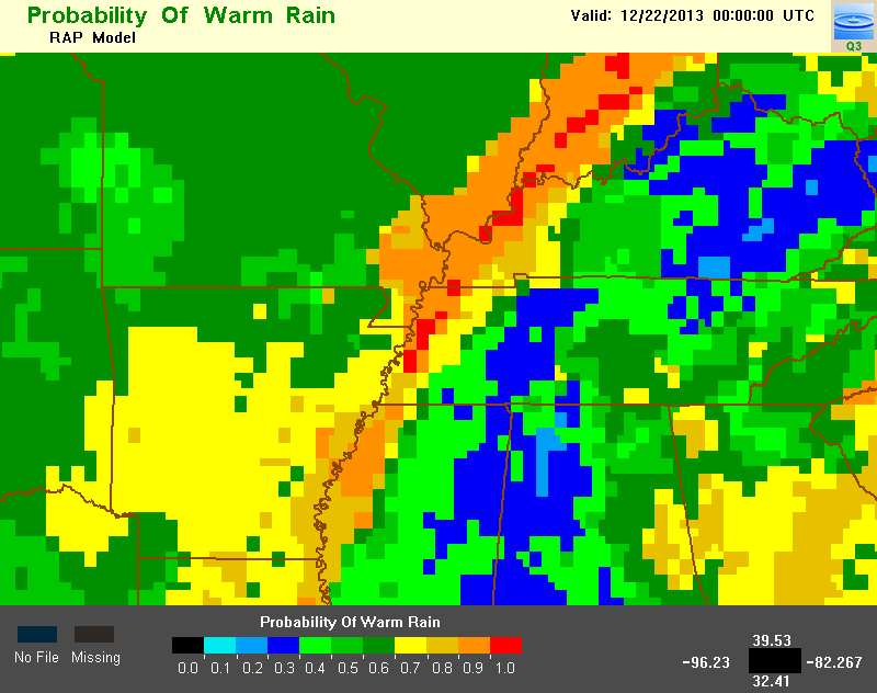
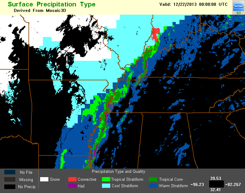
The POWR is used as a criterion for defining tropical rain in the Surface Precipitation Type product, via the Tropical Rain Identification algorithm. Figure 2 is an example image of (a) composite reflectivity, (b) POWR, and (c) the resulting Surface Precipitation Type product at 00Z on December 22, 2013. Notice how the high POWR regions were given one of the two tropical classifications. Additionally, POWR is used to define tropical-related Z-R relationships in the Surface Precipitation Rate product.
Example Images