I've come to realize that the different methods for data weighting in Stock Synthesis are not adequately documented and are the source of much confusion. Here's an overview of three methods for tuning the age and length composition sample sizes in SS description of the implementation, associated diagnostics, and challenges.

I personally see lots of benefit in the newest method, the Dirichlet-Multinomial, but it has not yet been widely used so there may be challenges in being an early adopter. Users should consider compare the results of multiple tuning methods.

Please reply with any questions or suggestions here so that we could refine some version of this text for inclusion in future versions of the User Manual.

In the future I will post a separate message about weighting indices of abundance and other tuning steps.

Overview

Note: in 2015 there was a CAPAM workshop dedicated to data-weighting. Description of the workshop is at http://www.capamresearch.org/data-weighting/workshop. The presentations from the workshop are available through that website and many of them were included in a special issue of Fisheries Research at https://www.sciencedirect.com/journal/fisheries-research/vol/192.

Three main methods for weighting length and age data have been used with Stock Synthesis:

1. McAllister-Ianelli
   Effective sample size is calculated from fit of observed to expected length or age compositions. Tuning algorithm is intended to make the arithmetic mean of the input sample size equal to the harmonic mean of the effective sample size.
   Reference:
   McAllister, M.K. and J.N. Ianelli 1997. Bayesian stock assessment using catch-age data and the sampling - importance resampling algorithm. Can. J. Fish. Aquat. Sci, 1997, 54(2): 284-300, https://doi.org/10.1139/f96-285 (PDF available at https://www.afsc.noaa.gov/refm/docs/pubs/McalisterIanelli97.pdf)

2. Francis
   Based on variability in the observed mean length or age by year, where the sample sizes are adjusted such that the fit of the expected mean length or age should fit within the uncertainty intervals at a rate which is consistent with variability expected based on the adjusted sample sizes.
   Reference:
   Francis, R.I.C.C. (2011). Data weighting in statistical fisheries stock assessment models. Can. J. Fish. Aquat. Sci. 68: 1124-1138. https://doi.org/10.1139/f2011-025. (It’s method “TA1.8”)

3. Dirichlet-Multinomial
   A new likelihood (as opposed to the standard multinomial) which includes an estimable parameter (theta) which scales the input sample size. In this case, the term “Effective sample size” has a different interpretation than in the McAllister-Ianelli approach.
   References:
   Thorson, J.T., Johnson, K.F., Methot, R.D. and Taylor, I.G. 2017. Model-based estimates of effective sample size in stock assessment models using the Dirichlet-multinomial distribution. Fish. Res. 192: 84-93. https://doi.org/10.1016/j.fishres.2016.06.005
   Thorson, J.T. 2018. Perspective: Let’s simplify stock assessment by replacing tuning algorithms with statistics. Fish. Res. https://doi.org/10.1016/j.fishres.2018.02.005

Applying the methods

McAllister-Ianelli

Implementation: The “Length_Comp_Fit_Summary” and “Age_Comp_Fit_Summary” sections in the Report file include information on the harmonic mean of the effective sample size and arithmetic mean of the input sample size used in this tuning method. In r4ss package, these tables are returned by the SS_output function as $Length_comp_Eff_N_tuning_check and $Age_comp_Eff_N_tuning_check.

A convenient way to process these values into the format required by the control file is to use the function
SS_tune_comps(replist, option = "MI")
where the input “replist” is the object created by SS_output. This function will return a table and also write a matching file called “suggested_tuning.ss” to the directory where the model was run.

For models using SS 3.30, the table created by SS_tune_comps can be pasted into the bottom of the control file in the section labeled “Input variance adjustments”, followed by the terminator line which indicates the end of the section. Here's an example of the first few rows of the table followed by the terminator line (not added by the function):

#Factor Fleet New_Var_adj hash Old_Var_adj New_Francis   New_MI Francis_mult Francis_lo Francis_hi  MI_mult Type   Name
      4     1    0.583669    #           1    0.273863 0.583669     0.273863   0.171537   0.620156 0.583669  len Fleet1
      4     2    0.786706    #           1    0.179728 0.786706     0.179728   0.122616   0.414949 0.786706  len Fleet2
      4     3    0.293040    #           1    0.144555 0.293040     0.144555   0.087435   0.371817 0.293040  len Fleet3
...
  -9999     0           0    # terminator line
 

Also see the help page for the r4ss function SS_varadjust which can be used to automatically write a new control file if you want to streamline the process of applying multiple iterations of this tuning method.

Diagnostic: If the tuning has been implemented, the green lines in the figure below would intersect at a point which is on the black 1-to-1 diagonal line in this figure created by the r4ss function SS_plots.

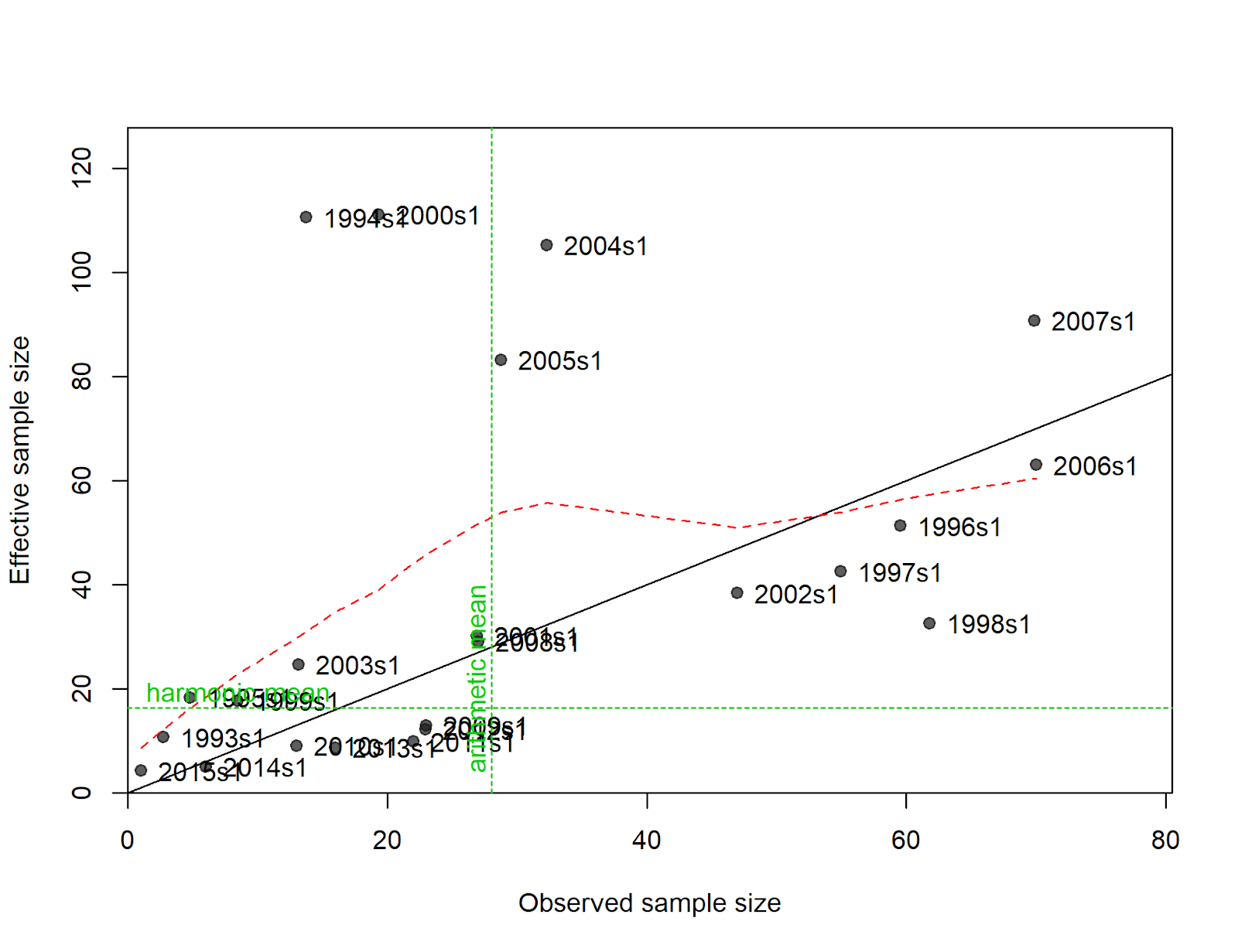
Figure: N-EffN comparison, Length comps, whole catch, Fleet1

Challenges:

• Subjective choice of how many iterations to take to achieve adequate convergence. Often just one iteration is applied.

• Takes time to implement so tuning is rarely repeated during retrospective or sensitivity analyses.

Francis

Implementation: recommended adjustments are calculated by the r4ss functions SSMethod.TA1.8 and SSMethod.Cond.TA1.8. These functions are rarely used alone but are called by the SS_plots function when making plots like the one below. For SS 3.30 models, the simplest way to get the adjustments in the format required by the control file is to use the SS_tune_comps function (described above under the McAllister-Ianelli method), but with a different option specified:
SS_tune_comps(replist, option = "Francis")

Diagnostic: The figure below shows the estimated 95% intervals around the observed mean length by year based on the input sample size (thick lines) and the increase in that uncertainty which would occur if the sample sizes were adjusted according to the proposed multiplier.

Figure: Mean length for Fleet1 with 95% confidence intervals based on current samples sizes. Francis data weighting method TA1.8: thinner intervals (with capped ends) show result of further adjusting sample sizes based on suggested multiplier (with 95% interval) for len data from Fleet1: 0.2739 (0.1661-0.6305)

Challenges:

• Subjective choice of how many iterations to take to achieve adequate convergence. Often just one iteration is applied.

• Takes time to implement so tuning is rarely repeated during retrospective or sensitivity analyses.

• Recommended adjustment can be sensitive to outliers (remove a few years of anomalous composition data can lead to large change in recommended adjustment)

Dirichlet-Multinomial

Implementation:

Change the choice of likelihood and set parameter choices in the data file

• In the specification of the length and/or age data, change "CompError" column in age and length comp specifications from 0 to 1 and "ParmSelect" from 0 to a sequence of numbers from 1 to N where N is the total number of combinations of fleet and age/length.

• Resulting input should look something like
  #_mintailcomp addtocomp combM+F CompressBns CompError ParmSelect minsamplesize   
  -1            0.001     0       0           1         1          0.001   #_fleet:1
  -1            0.001     0       0           1         2          0.001   #_fleet:2

• The ParmSelect column can also have repeated values so that multiple fleets share the same log(theta) parameter.

• If you have both length and age data, the ParmSelect should have separate numbers for each, e.g. 1 and 2 for the length comps and 3 and 4 for the age comps for the same two fleets.

Add parameter lines to the control file

• Add as many parameter lines as the maximum numbers in the ParmSelect column. The new parameter lines go after the main selectivity parameters but before any time-varying selectivity parameters

• Jim Thorson initially recommended bounds of -5 to 20, with a starting value of 0
  (which corresponds to a weight of about 50% of the input sample size). However, parameter estimates above 5 are associated with 99-100% weight with little information in the likelihood about the parameter value. Therefore, an upper bound of 5 may help identify cases that otherwise would have convergence issues.

• Example parameter lines are below (columns 9-14 not shown)
  #_LO    HI INIT    PRIOR PR_SD PR_type PHASE   env-var ... # parm_name
  -5      5  0.5     0     99    0       2       0       ... # ln(EffN_mult)_1
  -5      5  0.5     0     99    0       2       0       ... # ln(EffN_mult)_2

• Reset any existing variance adjustments factors that might have been used for the McAllister-Ianelli or Francis tuning methods. In 3.24 this means setting the values to 1, in 3.30, you can simply delete or comment-out the rows with the adjustments.

Diagnostic: The SS_output function in r4ss returns table like the following:

$Dirichlet_Multinomial_pars
                  Value Phase Min Max    Theta Theta/(1+Theta)
ln(EffN_mult)_1 -0.2219     2  -5  20  0.80097         0.44474
ln(EffN_mult)_2  2.3512     2  -5  20 10.49826         0.91303

The ratio shown in the final column is the estimated multiplier which can be compared to the sample size adjustment estimated in the other tuning methods above (the New_Var_adj column in the table produced by the SS_tune_comps function in r4ss).

If the reported Theta/(1+Theta) ratio is close to 1.0, that indicates that the model is trying to tune the sample size as high as possible. In this case, the log(Theta) parameters should be fixed at a high value, like the upper bound of 20, which will result in 100% weight being applied to the input sample sizes. An alternative would be to manually change the input sample sizes to a higher value so that the estimated weighting will be less than 100%.

There is also information about this result produced in the plots created by the SS_plots function:

Challenges:

• Not yet widely used so little guidance is available

• Does not allow weights above 100% (by design) so it's not yet clear how best to deal with the situation when the estimated weight is close to 100%

• Parameterization has potential to cause convergence issues or inefficient MCMC sampling when weights are close to 100% (Jim Thorson has proposed a prior distribution that may help with this, but has not yet been tested).