Forecasting snow accumulation is a difficult task, and not just because initial observational uncertainties and subtle atmospheric processes can lead to major precipitation type and intensity forecast errors. The various NWP models and ensembles use different numerical methods and post-processing techniques, resulting in important differences in how snow accumulation products are derived. In addition, snowfall forecast graphics on AWIPS and found on various websites and social media platforms use different assumptions, which can create a lot of confusion and uncertainty. The purpose of this guide is to help forecasters learn the assumptions and limitations associated with the creation of snowfall accumulation forecast products derived from NWP models and ensembles.
In the following pages, you will learn more about the physical process associated with snow accumulation (part 1), uncertainties associated with how snow is measured (part 2), how numerical models determine precipitation type (part 3), how models internally calculate snowfall accumulation (part 4), and how AWIPS and websites create snowfall accumulation graphics (part 5). Finally, there is a reference document for how different models parameterize, calculate, and produce output for snowfall (part 6). This guide is intended to be a living document, and changes will be incorporated as they are documented.
This guide is not intended to cover the broader topic of forecasting winter weather, but instead focuses on snow accumulation products derived from NWP models and ensembles. For more a more comprehensive overview of forecasting hazardous winter weather, visit theWarning Decision Training Division’s Winter Warning Operations Course.
2. How Snow Accumulates
Before we go into the assumptions used by NWP models, ensembles, and snow accumulation products, we need to go over some important physical details on how snow accumulates. Multiple factors can modulate how snow will accumulate as it falls from the cloud and reaches the ground. These factors are described below.
Crystal Type(s):
Given the same liquid water equivalent, snow accumulation characteristics at the surface depend heavily on the type of snow crystal(s) present. The type(s) of crystals are governed by the temperature and humidity characteristics of the environment as shown in the figure at right. Snow crystals can be broken down into two major types: plates and columns.
Plates include dendrites (high humidity environment) and solid plates (lower humidity environment). Dendrites are composed of many branches with air trapped between the barbs. The larger the dendrites/aggregates of dendrites, the larger the air-to-snow ratio and the greater potential snow depth upon accumulation at the surface. Solid plates, on the other hand, have no branches with trapped air and will pile up to less depth at the surface. Therefore, according to the figure, knowledge of the atmospheric moisture content is important to determine whether solid plates or dendrite are more likely.
Columns, including needles, tend to settle on the ground with little air between adjacent crystals, particularly as they are compressed, so the snow depth is generally less compared to dendrites and solid plates.
Fig: For similar amounts of liquid equivalent precipitation, different crystal types accumulate to different snow depths on the ground. Dendrite crystals tend to have a lot of air caught inside their branches, leading to the greatest snow depth of all the crystal types (1st and 2nd columns). This is followed by plates (4th column), and finally, needles/columns (3rd column). As it accumulates deeper, compaction becomes significant over time for snow composed primarily of dendrite crystals. Press the play button to visualize. Credit: The COMET Program at UCAR.
Aggregation:
Aggregation refers to the collection of two or more snow crystals which collide and join together during development in the cloud and/or descent to the surface. This can result in very large particles. A heavy fall of large dendrite aggregates can pile up to great depths quickly due to all of the air that becomes trapped between the branches of the aggregates. On the other hand, solid plates, needles, and other columns do not aggregate as readily when they collide since they don't have branches/barbs.
Riming:
Riming is a specific type of aggregation. Snow crystals can accrete supercooled liquid during descent through a warm cloud layer. Since rime ice results in less air in the branches of dendrites, the snow accumulation will be less than would be expected with the same crystals not subjected to riming.
Fig: Dendrite crystal branches tend to fracture in windy or turbulent conditions, lowering the potential snow depth at the surface. Press the play button to visualize. Credit: The COMET Program at UCAR.
Wind/Turbulence:
Complex dendrite crystals with many branches and barbs are quite fragile. In windy and/or turbulent conditions, the flakes are apt to collide as they form and fall from their source. The branches and barbs of the dendrites tend to break off during these collisions. Since these fractured crystals will pile up with less air between the branches than more pristine dendrites, the result is less accumulation in windy or turbulent conditions than in calm conditions with comparable thermodynamic profiles, as there is less air caught in the accumulated pile of snow.
Even if it is not windy as the snow falls, after accumulating on the surface, blowing snow along the ground can break off branches and barbs on dendrites, causing the snow to settle on the ground at less depth than before the wind started.
Wind Drift:
As the snow falls from its source, strong winds can blow the crystals downwind in their journey between the cloud and the ground. In a large storm system with mostly uniform precipitation, this effect would generally be negligible. But when the snow falls in a narrow band or in convective cells, strong winds in the subcloud layer can displace the location of resulting accumulation on the ground. This will generally not be captured in NWP output.
3. Snow Measurement Uncertainty
Even with perfect knowledge of snow accumulation processes, there is considerable uncertainty associated with the measurement of snow accumulation on the ground. It is usually impossible to measure snow perfectly to a tenth of an inch – or in a major storm, even to the nearest inch! Measurement of snow accumulation after it reaches the ground is modulated by several factors:
Surface type:
Ideally, snow accumulation reports would all be sourced from measurements made on a properly-sited white snowboard. Meteorologists might accept snow reports from other types of surfaces in order to achieve a greater geographic density of reports, at the expense of more uncertainty. A typical source of reporting error is the type of surface on which the snow measurement is made. Snow accumulating on top of thick grass might lead to measurement of both the height of the grass and the snow on top of it, not just the snow. Snow accumulating on asphalt, dirt, a brown wooden deck, or on top of a vehicle, might experience more melting in marginal temperature environments than an adjacent snow board, especially if the snow falls soon after warm temperatures or sunny conditions. Snow measurements taken under trees would cause an artificially low surface measurement. NWP output generally does not attempt to modulate snow accumulation amount by land surface type (though most will accumulate snow on top of ice on bodies of water analyzed to be frozen).
Frequency of measurement:
One critical factor in snow accumulation verification is the frequency of measurement. During heavy snowfall, snow compaction can occur quickly, so summing measurements made every hour for 24 hours could yield a much higher result than a single measurement made at the end of 24 hours. Melting and/or sublimation are also processes which can reduce the amount of snow on the ground if measurements are taken infrequently. Windy conditions might cause snow to drift on or blow away from the measurement site over time. It is important snow accumulation measurements are made as soon as possible at the end of a storm and the user knows how often measurements were made by an observer over the course of a storm.
Compaction:
As falling snow accumulates on the ground, the weight of the new snow on top will compress the older snow below, a process known as compaction. Even after the snow ends, gravity gradually compresses the layer of snow into a thinner layer. Strong winds at the surface can promote drifting and compaction. Measurement frequency, and how quickly after the storm the snow accumulation is measured, are both critical to keep uncertainties associated with compaction to a minimum. NWP and post-processing methods vary on how they handle compaction.
NWS Snow Measurement Guidelines
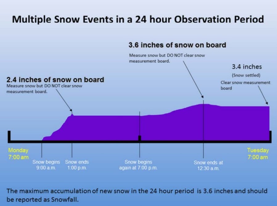
The official NWS Snow Measurement Guidelines state measurements should be taken on a white snow board away from obstructions. The board should be cleared at least once every 24 hours, and ideally once every 6 hours, but not more frequently. Supplemental measurements may be made without clearing the snow board to determine the maximum depth on the board, as illustrated in the figure.
When verifying forecasts and reporting snow amounts, consideration should be given to whether reports received have followed this standard.
Drifting:
During or after the snowfall, high winds at the surface can cause considerable drifting. This can make precise measurement difficult to impossible for an observer. Snow accumulation reports from untrained observers might not take into account the need to measure the snow on flat ground away from objects and obstructions, nor the need to calculate the average of multiple dispersed measurements when not using a snowboard. NWP output approximates the average snow accumulation amount over wide areas, not attempting to model drifting.
Fig: In this example, the snow depth decreases over time from two processes: melting into the ground from below and sublimation from the top. Press the play button to visualize. Credit: The COMET Program at UCAR
Melting:
Melting of snow after it reaches the ground can occur in several ways. First, snow falling on warm surfaces can melt on contact. Even if snow is accumulating quickly, a warm surface can gradually transfer its heat to the snow at the point of contact, melting the snow layer from below. During compaction, snow at the bottom of a layer can melt as the air it contains is warmed under greater air pressure (ideal gas law). When the air temperature warms above freezing, the snow on the ground will begin a phase change from solid to liquid, with the water either soaking into the ground or running off, decreasing its depth.
Sublimation:
When the air is sufficiently dry and below freezing, a phase change will occur for snow on the ground directly from ice to water vapor in a process called sublimation. This will gradually decrease the depth of the snow. Sublimation is the most efficient on sunny, dry, windy days.
4. Numerical Methods For Determining Precipitation Type
This section describes numerical methods models, algorithms, and humans can use to determine precipitation type. These use a variety of approximations and physical assumptions which vary based on the thermodynamic setup. Given the various sensitivities to precipitation type -- e.g., precipitation rate, convection, hydrometeor size, presence of a warm nose and/or cold dome, etc. -- ideally a multi-method ensemble approach would be used in a probabilistic framework.
Rudimentary Thermodynamic Profile Techniques
These techniques are generally not used any more in numerical models and post-processing algorithms, but are still sometimes used by human forecasters for a quick judgment on possible precipitation type.
Pressure Layer "Thickness" Techniques:
These simple techniques based on temperature profiles were created from rules-of-thumb in times of limited computing capabilities to quickly delineate regions of snow, so the user can then go on to estimate snow amounts. These can be generally categorized into two types:
Deep Layer (1000-500 hPa): Areas with deep layer thickness less than a certain depth are often approximated to be completely below freezing, so snow is assumed to be the primary precipitation type (usually, 5400 m is used near sea level)
Partial Layer (usually 1000-850 hPa or 850-700 hPa): Different thickness values for each layer can indicate what type of precipitation (snow, sleet, rain, freezing rain, or a mix of types) may occur since thickness relates to temperatures in each layer
Was developed for southeastern Canada but is sometimes used in the northeastern US (See Cantin and Bachand 1993)
Limitations:
Uses a single thickness value to approximate the layer's maximum temperature, not accounting for the actual temperature profile - so it can fail to account for shallow atmospheric layers above freezing, overestimating areal snow coverage
Does not account for the moisture profile; for example it would miss evaporative cooling potential in a dry air mass
Critical thickness values can vary by elevation
"Top-Down" Methods:
Various techniques using the thermodynamic profile (dry-bulb temperature and dewpoint, wet-bulb temperature, or relative humidity) above a given point, starting from the level of precipitation particle development and going down, to determine the surface precipitation type at that point.
Limitations:
Doesn't account for vertical motion which can change the local thermodynamic profile
If a dry-bulb temperature profile is used, would not account for evaporative cooling in a dry air mass
Does not account for melting and refreezing from smaller cold layers, it is solely based on maximum temperature of a warm nose and minimum temperature of the cold dome below.
This technique uses the wet bulb temperature profile in model post-processing to create a mini-ensemble of precipitation type outcomes at the surface based on different methods.
The majority of techniques in the mini-ensemble determines the surface precipitation type
If there is a tie, the precipitation type is determined in order from most to least "hazardous" as follows: Freezing Rain > Snow > Sleet > Rain
Limitation: Although this uses a mini-ensemble approach in post-processing, this method does not account in any way for synoptic/mesoscale uncertainty. This approach only attempts to capture the uncertainty associated with how different schemes handle wet bulb temperature profiles to determine surface precipitation type.
Advanced technique that predicts mixing ratios of five liquid/ice species: cloud water, rain, cloud ice, snow, and graupel AND the number concentration of cloud ice
Provides much more accurate precipitation type and QPF amounts by breaking out different types of precipitation within the model output, yielding a better snow forecast
Limitation: it is still a parameterization, therefore it is not fully representing actual physical processes
Global Systems Division (GSD) Thompson scheme (for HRRR/RAP) (DTC/CCPP Reference)
More advanced than the original Thompson 2008 scheme by including aggregation of liquid and freezing precipitation in cloud
Includes/allows for supercooled water droplets in-cloud improving growth/aggregation rates and types
Limitation: Though slightly improved, it is still a parameterization, therefore it is not fully representing actual physical processes
The original method looks at the vertical temperature profile to determine areas above and below 0°C which, along with mean thickness temperatures, are used to determine magnitude of melting and refreezing, and then uses surface temperature and dewpoint to determine a final categorical precipitation type/mixture among these choices: Snow, Rain, Freezing rain, Sleet, Mixed rain/snow, Mixed freezing rain/sleet
The Revised Bourgouin Method implements several improvements:
A larger developmental and independent dataset
Use of wet-bulb temperature profiles
Ability to diagnose freezing precipitation in situations without ice nucleation, improving overall prediction of freezing rain events
Probabilistic output that accounts for uncertainties in the spectrum of hydrometeor sizes, forecast or observed soundings, and space and time
Allowance for all combinations of wintry mixes
Limitation:Both methods will struggle with rapid temporal and/or spatial variations in the thermodynamic profile (often the case around convective precipitation)
5. Numerical Methods For Determining Snow Accumulation
This section describes various methods used by models and post-processing techniques to accumulate snow at the surface. The techniques described below generally do not account for what happens to the snow after it reaches the ground, except where noted. Light snow falling onto a very warm surface might melt on contact completely, while snow falling at a heavier rate onto the same surface might cool the surface to freezing more rapidly, allowing accumulation to commence more quickly.
Users should be cognizant of the length of time represented in a snow accumulation graphic from a model or post-processing technique. With heavy snow falling over a long period, reduction of snow depth at the surface due to compaction would not be accounted for in some of these techniques. A warm air mass moving in or a high solar angle close to the vernal or autumnal equinox might lead to partial or complete melting with time not accounted for in these calculations. Even in cold conditions, a dry air mass moving in under sunny skies would encourage the sublimation process, reducing the snow depth at the surface over time.
Constant Snow:Liquid Ratio (SLR) Techniques
This simple technique multiplies the Quantitative Precipitation Forecast (QPF) or Snow Water Equivalent (SWE) by a fixed number to get a snow amount.
For example, a constant 10:1 SLR would yield 1" of snow for 0.1" of QPF or SWE. A constant 15:1 SLR would yield 1.5" of snow for the same 0.1" of QPF or SWE. The constant SLR to be used is determined by thickness values and/or the maximum temperature in the column. Lower SLRs (5:1 or 8:1) are often observed in marginally-warm environments or where sleet mixes with the snow. Higher SLRs (15:1 or 17:1) are often observed in very cold environments.
Limitation: the SLR is not uniform geographically or even in the same event at a fixed location. Different thermodynamic profiles can significantly affect the SLR (See Baxter et al. 2005), yielding potentially-substantial errors when using a constant SLR.
This technique identifies the maximum temperature (Tmax) in the column from the surface to 500 hPa:
If Tmax is greater than 271.16K (~28°F or -2°C), SLR = 12 + 2(271.16-Tmax)
If Tmax is less than or equal to 271.16K, SLR = 12 + (271.16-Tmax)
Assuming primarily dendritic snow, this is generally superior to constant 10:1 SLR in areas of marginally warm or very cold temperature profiles
Limitation: Can substantially overestimate accumulation in very cold air masses with strong winds/turbulence, as crystal branches break off due to collision of dendrites during descent, lowering the density of the accumulated snow at the surface
This technique uses hourly model data and combines multiple techniques at a single point (Cobb and Waldstreicher 2005):
Looks at vertical velocity, wet- and dry-bulb temperatures, and relative humidity to create SLR at every model level from where the hydrometeor initiates to the surface
Calculates percentage of hydrometeors reaching the surface along with precipitation type and SLR at the lowest model level
Precipitation types are binned into snow, ice (sleet), or liquid (rain/freezing rain)
This technique is difficult to implement within model code, so it is generally done in model post-processing
A modification to the Cobb method is applied when using data from Convection Allowing Models to account for stronger vertical velocities in those models
Artificial Neural Network technique using 28 radiosonde sites collocated with surface reports to from a dataset spanning 1973-1994
Looks at low-to-mid level temperature and relative humidity, mid-to-upper level temperature, mid and upper level relative humidity, and the month (which is a proxy for insolation)
Attempts to account for compaction using surface wind speed and liquid precipitation estimation
Breaks out light/moderate/heavy snow density
Limitation: Neglects in-cloud vertical motion, strong low-level wind, and early/late season ground temperature effects (like warm ground, wet snow)
6. NWP Snow Accumulation Products
What you see in AWIPS, WSUP, and various websites is usually not straight from the model! Only the HRRR and RAP produce explicit snowfall output (and most websites don't display it). The other NCEP models produce a snow water equivalent (SWE) product, but AWIPS and most graphics on the web use the QPF output instead of SWE.
The ECMWF and Environment Canada models keep track of precipitation type during each model step but then output an overall SWE covering multiple hours, and end users (AWIPS and websites) have to convert to snow accumulation on their own.
Below are how various model snow accumulation product displays are derived:
AWIPS Snow Accumulation Product
The AWIPS baseline software produces snow accumulation plots/graphics using an outdated thickness-based method. Bottom line -- DO NOT USE in and around marginally-warm thermodynamic environments and in mixed precipitation areas! There are often significant differences seen in AWIPS plots compared to what various websites (rapidrefresh.noaa.gov, pivotalweather, etc.) plot.
The issue revolves around how AWIPS processes the data. For most models (except NBM), the AWIPS snow accumulation products use "rules of thumb" techniques that are 25+ years old. For all models except the NBM, AWIPS snow accumulation maps are:
Using model QPF and NOT snow water equivalent
Calculating on-the-fly based on model 1000-500 hPa thickness and surface topography/elevation (NOT temperature profiles!)
Employing one of four possible Snow:Liquid Ratio (SLR) calculations at each grid point based on thickness:
SLR 0:1 (thickness implies too warm for snow)
SLR 5:1 (thickness implies marginal liquid/snow and/or presence of sleet)
SLR 10:1 (thickness implies cold enough for all snow)
SLR of 15:1 (thickness implies very cold air mass)
SLR category adjusted upward at higher elevations
Multiplying the QPF by the calculated SLR in CAVE/D2D to produce contour/image plot
NOTE: This does NOT impact the raw model data. As a workaround, you can load individual hours into GFE and view the output there to see what the models may be forecasting for snowfall, but when producing final grids, use of standard regional or national tools designed for spatial consistency is recommended (e.g., ForecastBuilder).
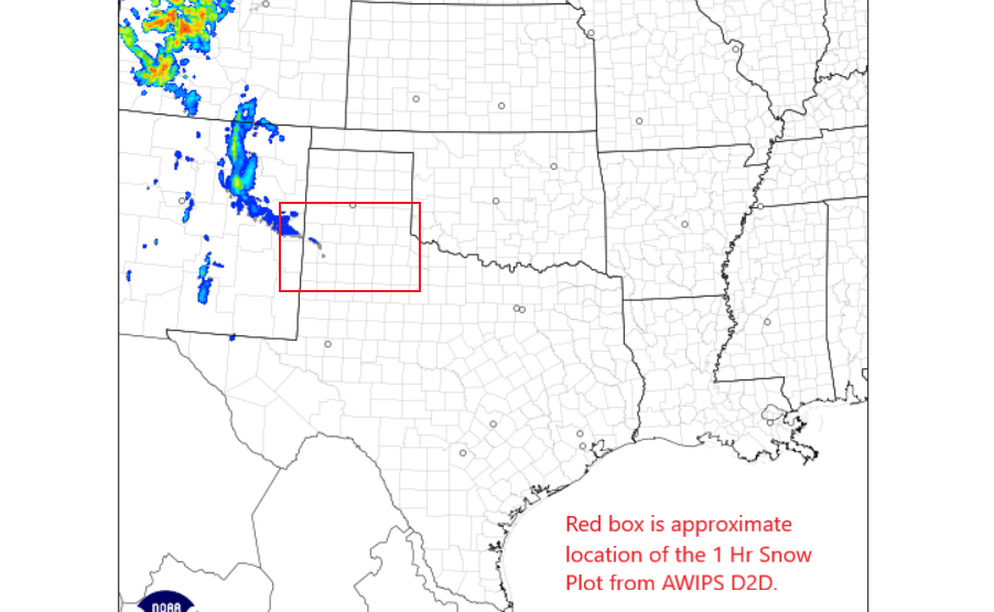
The 1 hour forecast graphic of Snow Accumulation Using Thickness from AWIPS shows a swath of 2-4" snowfall surrounded by a large area of 1-2" across parts of the west Texas. Note the artificial discontinuities in snowfall where the AWIPS algorithm tries to take into account changes in elevation.
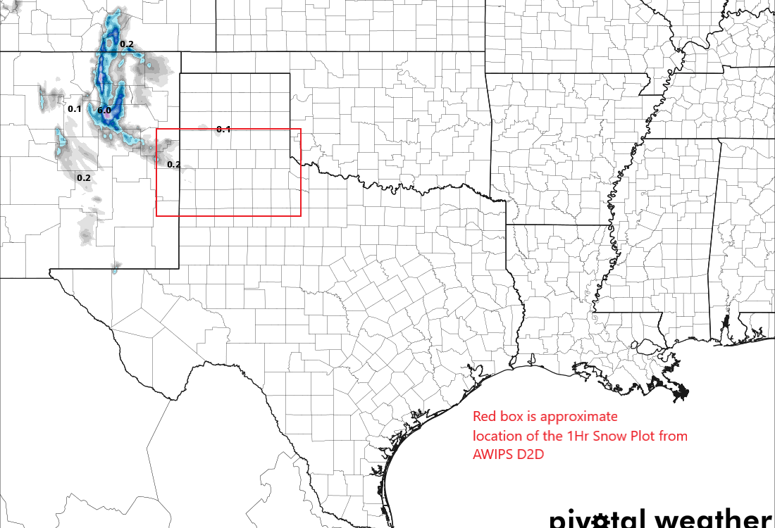
The snow depth reported from the HRRR barely breaks 0.1" anywhere in the area of the 1-4" of snow accumulation depicted in the AWIPS product.
The output from this external website is similar to the rapidrefresh.noaa.gov site, so confidence is high that the AWIPS method is producing unreasonable output.
Model Snow Water Equivalent Product
Post-produced by NCEP for most of their models (GFS, GEFS, NAM, and HiResW, but NOT the HRRR/RAP), the snow water equivalent (SWE) product attempts to determine what proportion of the precipitation produced by the model will be snow upon reaching the surface, which can then be converted to snow accumulation using one of the techniques below. This is more advanced than simple thickness/elevation techniques applied to QPF, but is still limited by the inability to separate ice and/or freezing rain.
Does attempt to take into account surface processes (melting, sublimation, and compaction) in each model time step
Output every hour
Available in AWIPS through the Volume Browser or Product Browser but is displayed in liquid equivalent amount
Users must apply their own SLR to SWE to get a snowfall accumulation amount
Snow and sleet are tallied together
Does not separate out freezing rain
Some external websites use SWE to create their snowfall graphics, but most use QPF (check with website)
Constant 10:1 SLR Product
Not currently available in AWIPS but ubiquitous on websites
Most websites use QPF, some attempt to use SWE if available
Multiplies model QPF or SWE by 10 to get snowfall in areas deemed cold enough for snow
Methods for determining snow vs. rain temperature profile vary by website
Multiple of 10 or nothing, so will overestimate snow in marginally-warm temperature environments and underestimate snow in very cold air masses containing dendrites
Websites will often categorize sleet as 10:1 snow, causing potentially-significant overestimation where sleet mixes in or is the primary precipitation type
Kuchera Product
Not available in AWIPS but available on many external websites
Uses a simple variable density formula to determine SLR based on maximum temperature in the column (Tmax):
If Tmax > 271.16 K: SLR = 12 + 2(271.16-Tmax)
If Tmax <= 271.16 K: SLR = 12 + (271.16-Tmax)
Does a good job lowering SLR in marginally-warm environments and raising SLR in very cold environments where dendrites are expected
However, it does not take into account the breaking off of dendrite branches during descent in windy conditions, so it can overestimate snow accumulation in very cold and windy environments (blizzards)
Can still capture some freezing rain or sleet as snow, but generally at lower amounts than constant 10:1 or thickness-based methods
Most external websites use QPF to multiply with the SLR, some attempt to use SWE if available (check with website)
Generally captures gradients in accumulation well in environments with temperature gradients during dendrite-predominate snow events
Snow Depth Product
Directly produced by the HRRR and RAP, this uses a simplistic SLR that is a function tied only to the 2 meter temperature
SLR and melting are assessed at each model time step which usually provides better accumulations compared to other post-processed products like Kuchera, thickness, constant 10:1, etc.
Depth is updated at 00 UTC with a blend of the 23km USAF snow depth field and 6-hour forecasted snow depth from the previous cycle (so, for example, the 6 hour forecast from the 18 UTC run for the 00 UTC run initialization)
Once the model has started running, snow cover and water equivalent snow depth are allowed to evolve, affecting albedo for radiative transfer and impacting the surface/land interaction. This will change the water equivalent snow depth but does not explicitly produce snow depth (must use conversions!)
NAM starts the same as the GFS with the USAF analysis, but also uses the 4 km daily NESDIS northern hemisphere snow cover analysis and is updated daily with data valid as of 18 UTC, and is available in time for the 06 UTC and later runs of the model
Once the model has started running, NAM microphysics takes into account fractional snow amounts (to separate snow from rain), albedo, snowmelt, and sublimation
Model tries to take into account new snow density from air temperature in the first layer and surface temperature -- a rough proxy to account for compaction
Boundary layer microphysics scheme also tries to account for heat flux and sublimation over time, with surface land model used for ground temperature
Change-in-Snow Depth Product
Produced by many websites, this is simply the net positive increase in snow depth reported from the model over the indicated time duration
Does not take into account any negative contributions to depth over time such as melting or rain falling on top of snow, nor compaction or drifting
Does not take into account freezing rain or sleet mixing with falling snow
Often found to be the best representation of verifying storm total snow accumulation in events where precipitation type is not a source of uncertainty
A Note on NOHRSC Products
NOHRSC snow depth products feed into most models to initialize surface snow cover.
This can have a big effect on 2 meter/surface temperature forecasts, so check satellite imagery to estimate actual snow surface cover and compare against model snow depth displays at the same time step
In many areas, the NOHRSC analysis relies on automated remote liquid precipitation sensors where an estimated SLR is applied
Baldwin, M. and S. Contorno, 1993: Development of a weather-type prediction system for NMC's mesoscale ETA model. Preprints, 13th Conf. on Weather Analysis and Forecasting, Vienna, VA, Amer. Meteor. Soc., 86–87.
Cobb, D. and J. Waldstreicher. 2005: A Simple Physically Based Snowfall Algorithm. Preprints,21st Conference on Weather Analysis and Forecasting/17th Conference on Numerical Weather Prediction, Washington, DC, Amer. Meteor. Soc.
Nakaya, U., 1954: Snow Crystals: Natural and Artificial. Harvard University Press.
Ramer, J., 1993: An empirical technique for diagnosing precipitation type from model output. Preprints,Fifth Int. Conf. on Aviation Weather Systems, Vienna, VA, Amer. Meteor. Soc., 227–230.


 Forecasting snow accumulation is a difficult task, and not just because initial observational uncertainties and subtle atmospheric processes can lead to major precipitation type and intensity forecast errors. The various NWP models and ensembles use different numerical methods and post-processing techniques, resulting in important differences in how snow accumulation products are derived. In addition, snowfall forecast graphics on AWIPS and found on various websites and social media platforms use different assumptions, which can create a lot of confusion and uncertainty. The purpose of this guide is to help forecasters learn the assumptions and limitations associated with the creation of snowfall accumulation forecast products derived from NWP models and ensembles.
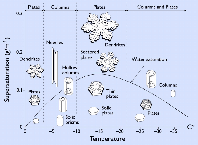
 The official